Make an initial guess of C4 hyperbola parameter values for one curve

Creates a function that makes an initial guess of C4 hyperbola model parameter values for one curve. This function is used internally by fit_c4_aci_hyperbola.

Values estimated by this guessing function should be considered inaccurate, and should always be improved upon by an optimizer.

Usage

initial_guess_c4_aci_hyperbola(
    a_column_name = 'A'
  )

Arguments

a_column_name

The name of the column in rc_exdf that contains the net assimilation rate in micromol m^(-2) s^(-1).

Details

Here we estimate values of c4_curvature, c4_slope, rL, and Vmax from a measured C4 CO2 response curve. For more information about these parameters, see the documentation for calculate_c4_assimilation_hyperbola.

Here we take a very simple approach to forming the initial guess. We always choose c4_curvature = 0.5, c4_slope = 1.0, and rL = 0.0. For Vmax, we use Vmax = max{A} - rL_guess, where max{A} is the largest observed net CO2 assimilation rate and rL_guess is the guess for rL.

Value

A function with one input argument rc_exdf, which should be an exdf object representing one C4 CO2 response curve. The return value of this function will be a numeric vector with four elements, representing the values of c4_curvature, c4_slope, rL, and Vmax (in that order).

Examples

# Read an example Licor file included in the PhotoGEA package
licor_file <- read_gasex_file(
  PhotoGEA_example_file_path('c4_aci_1.xlsx')
)

# Define a new column that uniquely identifies each curve
licor_file[, 'species_plot'] <-
  paste(licor_file[, 'species'], '-', licor_file[, 'plot'] )

# Organize the data
licor_file <- organize_response_curve_data(
    licor_file,
    'species_plot',
    c(9, 10, 16),
    'CO2_r_sp'
)

# Create the guessing function
guessing_func <- initial_guess_c4_aci_hyperbola()

# Apply it and see the initial guesses for each curve
print(by(licor_file, licor_file[, 'species_plot'], guessing_func))
#> $`maize - 5`
#> [1]  0.50000  1.00000  0.00000 67.33821
#> 
#> $`sorghum - 2`
#> [1]  0.50000  1.00000  0.00000 71.16098
#> 
#> $`sorghum - 3`
#> [1]  0.50000  1.00000  0.00000 69.62463
#> 

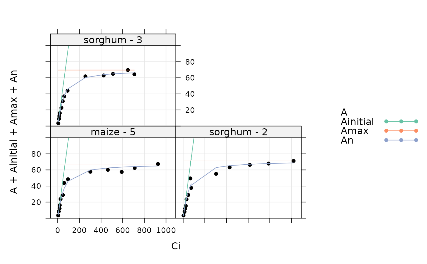
# A simple way to visualize the guesses is to "fit" the curves using the null
# optimizer, which simply returns the initial guess
aci_results <- consolidate(by(
  licor_file,
  licor_file[, 'species_plot'],
  fit_c4_aci_hyperbola,
  optim_fun = optimizer_null()
))

plot_c4_aci_hyperbola_fit(aci_results, 'species_plot', ylim = c(-10, 100))