Creating Your Own Processing Tools • PhotoGEA

Overview

The PhotoGEA package contains many functions for processing gas exchange data, such as apply_gm and fit_c3_aci. (A complete list is available in the Developing a Data Analysis Pipeline vignette.) However, you may wish to perform some kind of processing that is not already available from PhotoGEA. In this case, it is possible to create your own processing tools that will be compatible with the other functions in PhotoGEA that help with loading data, validating data, processing sets of multiple reponse curves, and analyzing the results.

In this vignette, we will provide an example showing some of the best practices for creating your own processing tools. If you create a tool that may be useful to others and you would like to share it, contact the PhotoGEA package maintainer about adding your function to the package.

Loading Packages

As always, the first step is to load the packages we will be using. In addition to PhotoGEA, we will also use the lattice package.

# Load required packages
library(PhotoGEA)
library(lattice)

If the lattice package is not installed on your R setup, you can install it by typing install.packages('lattice').

Loading and Validating Data

For this example, we will load the same set of C₃ A-Ci curves that are used in the Analyzing C3 A-Ci Curves vignette, and we will perform the same steps for organizing and cleaning the data. See that vignette for more details about these steps. For brevity, the commands are not included here, but they can be found at the end of this vignette in Commands From This Document.

Choosing a Model To Use

For this example, we will develop a function that fits a rectangular hyperbola to an A-Ci curve. A rectangular hyperbola is an equation of the form f(x) = y_max * x / (x + x_half). We can understand a great deal about this type of equation by examining its form:

When x is very large, x + x_half can be approximated as x, so in this case, the function reduces to y_max * x / x = y_max. In other words, the function reaches a constant value of y_max when x is large.
When x is x_half, the function’s value is y_max * x_half / (x_half + x_half) = y_max / 2. In other words, x_half is the value of x where the function reaches half of its maximum value.
When x is small, x + x_half can be approximated by x_half. In this case, the function reduces to y_max * x / x_half. In other words, the function is a straight line with slope y_max / x_half when x is small.
When x is exactly zero, the function is also zero.

With this in mind, we can see that a rectangular hyperbola begins with a linear portion and flattens out to a constant value. This is generally similar to the shape of an A-Ci curve, so it might be reasonable to use this equation for fitting. This type of model would be characterized as an “empirical” model (in contrast to a mechanistic or process-based model) because there is no underlying explanation for why this equation should be a good fit. Thus, it could be considered to be a simpler alternative to the Farquhar-von-Caemmerer-Berry model used in the fit_c3_aci function.

When applying this to an A-Ci curve, we will want to replace the independent variable x with Ci and the calculated value with the net assimilation A. One caveat is that A is generally negative when Ci is zero or very low, but the rectangular hyperbola never returns negative values. To get a better fit, it will be helpful to include respiration as a constant value subtracted from the hyperbola: A = A_max * Ci / (Ci + Ci_half) - Rd.

General Suggestions for PhotoGEA Fitting Functions

When creating a PhotoGEA fitting function, it is a good idea to follow these rules, which will ensure that the function is compatible with by + consolidate and has similar inputs and outputs to other fitting functions:

The first input argument should be an exdf object that represents one “unit” of data; in this case, a single A-Ci curve. This argument is often called replicate_exdf as a reminder of what it represents and what type of object it should be.
The first argument should be checked to make sure it is an exdf; this can be done using is.exdf.
The name of each important column from the exdf object should be passed as an input argument with a default value.
The function should check to make sure each important column is in the exdf object and that it has the expected units; this check can be accomplished with the check_required_variables function from PhotoGEA.
The function should return a list of named exdf objects as its outputs; most fitting functions return exdf objects called fits and parameters.
The fits return object should be a copy of the original data with additional columns for the fitted values and the fit residuals.
The parameters return object should have one row, and three different types of columns:
- Some of its columns should include identifying information about the curve such as species or event; this information can be obtained with the identifier_columns function from PhotoGEA.
- Some of its columns should include statistics that describe the quality of the fit, such as the root mean squared error; this information can be obtained with the residual_stats function from PhotoGEA.
- The other columns should include the best-fit values of the model’s parameters and any other information that may be important to the user.
Any exdf objects returned by the function should be fully documented with units for each relevant column.
The category for each exdf column created by the function should be set to its name to provide a record of how the column was calculated.
Any problems detected while checking the inputs should cause errors.
If a fit fails, the function should return NA results rather than causing an error. Otherwise, this will cause problems while fitting many curves at once, since the process will be disrupted by any errors that are thrown.
In general, the structure of the output (e.g. the number of exdf objects in the list, the names of the exdf objects in the list, and the columns in each exdf object) should always be the same, no matter what the function’s inputs are and no matter what the fitting results are. Any outputs that are not relevant for a particular fit should just be set to NA.
Provide default values for as many input arguments as possible. (No default should be provided for replicate_exdf, of course.)

In the next section, we will create a fitting function that meets these criteria.

Writing A Fitting Function

Here we write a function that fits a rectangular hyperbola to an A-Ci curve and follows the suggestions outlined above:

# Define a custom fitting function
fit_hyperbola <- function(
  replicate_exdf,
  a_column_name = 'A',
  ci_column_name = 'Ci',
  initial_guess = list(A_max = 40, Ci_half = 100, Rd = 1)
)
{
  ### Check inputs

  if (!is.exdf(replicate_exdf)) {
      stop("fit_hyperbola requires an exdf object")
  }

  # Make sure the required variables are defined and have the correct units
  required_variables <- list()
  required_variables[[a_column_name]] <- "micromol m^(-2) s^(-1)"
  required_variables[[ci_column_name]] <- "micromol mol^(-1)"

  check_required_variables(replicate_exdf, required_variables)

  # Extract the values of several important columns
  A <- replicate_exdf[, a_column_name]
  Ci <- replicate_exdf[, ci_column_name]

  ### Perform processing operations

  # Wrap `stats::nls` in a `tryCatch` block so we can indicate fit failures by
  # setting `aci_fit` to `NULL`.
  aci_fit <- tryCatch(
    {
      stats::nls(A ~ A_max * Ci / (Ci + Ci_half) - Rd, start = initial_guess)
    },
    error = function(cond) {
      print('Having trouble fitting an A-Ci curve:')
      print(identifier_columns(replicate_exdf))
      print('Giving up on the fit :(')
      print(cond)
      return(NULL)
    },
    warning = function(cond) {
      print('Having trouble fitting an A-Ci curve:')
      print(identifier_columns(replicate_exdf))
      print('Giving up on the fit :(')
      print(cond)
      return(NULL)
    }
  )

  ### Collect and document outputs

  # Extract the fit results and add the fits and residuals to the exdf object
    if (is.null(aci_fit)) {
        A_max <- NA
        A_max_err <- NA
        Ci_half <- NA
        Ci_half_err <- NA
        Rd <- NA
        Rd_err <- NA
        replicate_exdf[, paste0(a_column_name, '_fit')] <- NA
        replicate_exdf[, paste0(a_column_name, '_residuals')] <- NA
    } else {
        fit_summary <- summary(aci_fit)
        A_max <- fit_summary$coefficients[1,1]
        A_max_err <- fit_summary$coefficients[1,2]
        Ci_half <- fit_summary$coefficients[2,1]
        Ci_half_err <- fit_summary$coefficients[2,2]
        Rd <- fit_summary$coefficients[3,1]
        Rd_err <- fit_summary$coefficients[3,2]

        replicate_exdf[, paste0(a_column_name, '_fit')] <-
          A_max * Ci / (Ci + Ci_half) - Rd

        replicate_exdf[, paste0(a_column_name, '_residuals')] <-
          fit_summary$residuals
    }

    # Document the columns that were added to the replicate exdf
    replicate_exdf <- document_variables(
        replicate_exdf,
        c('fit_hyperbola', paste0(a_column_name, '_fit'),       'micromol m^(-2) s^(-1)'),
        c('fit_hyperbola', paste0(a_column_name, '_residuals'), 'micromol m^(-2) s^(-1)')
    )

    # Get the replicate identifier columns
    replicate_identifiers <- identifier_columns(replicate_exdf)

    # Attach the residual stats to the identifiers
    replicate_identifiers <- cbind(
        replicate_identifiers,
        residual_stats(
            replicate_exdf[, paste0(a_column_name, '_residuals')],
            replicate_exdf$units[[a_column_name]],
            3
        )
    )

    # Add the values of the fitted parameters
    replicate_identifiers[, 'A_max'] <- A_max
    replicate_identifiers[, 'A_max_err'] <- A_max_err
    replicate_identifiers[, 'Ci_half'] <- Ci_half
    replicate_identifiers[, 'Ci_half_err'] <- Ci_half_err
    replicate_identifiers[, 'Rd'] <- Rd
    replicate_identifiers[, 'Rd_err'] <- Rd_err

    # Document the columns that were added
    replicate_identifiers <- document_variables(
        replicate_identifiers,
        c('fit_hyperbola', 'A_max',       'micromol m^(-2) s^(-1)'),
        c('fit_hyperbola', 'A_max_err',   'micromol m^(-2) s^(-1)'),
        c('fit_hyperbola', 'Ci_half',     'micromol mol^(-1)'),
        c('fit_hyperbola', 'Ci_half_err', 'micromol mol^(-1)'),
        c('fit_hyperbola', 'Rd',          'micromol m^(-2) s^(-1)'),
        c('fit_hyperbola', 'Rd_err',      'micromol m^(-2) s^(-1)')
    )

    return(list(
      fits = replicate_exdf,
      parameters = replicate_identifiers
    ))
}

Here we have split the code into three main sections corresponding to the main steps that should be taken in any processing function:

Check inputs: Here we check the type of replicate_exdf and the units of any columns that will be accessed during the subsequent processing.
Perform processing operations: Here we actually perform the fit and get the results in their default form.
Collect and document outputs: Here we reorganize the fit results into two exdf objects corresponding to the fits and parameters, and make sure that all units are documented. This section ends by returning the results as a list of named exdf objects.

To make the fit, we have chosen to use nls, a function from base R that performs nonlinear least-squares fitting. This function is fairly straightforward to use, and it is quite popular. It requires an initial guess for the values of the model’s parameters, so an initial_guess input argument was included in fit_hyperbola allowing the user to specify the starting guess. One issue with nls is that it will throw an error if the fit is not successful. Dealing with these possible errors necessitates some extra code. First, we wrap the call to nls in tryCatch, and then later we have to decide what to return when there is a fit failure; here we just return NA for all the variables normally determined from the fitting procedure.

One improvement that could be made is to provide a way to generate a better initial guess for the starting parameter values, but we have left it out for brevity.

Using the Fitting Function

Now we can use the new fitting just as we would use any other processing function from PhotoGEA. Here we will use it to fit all the response curves in the example data set, and then examine the results by plotting the fits, plotting the residuals, and viewing the parameter values. These commands are nearly identical to ones from the Analyzing C3 A-Ci Curves vignette.

# Fit each curve
c3_aci_results <- consolidate(by(
  licor_data,                       # The `exdf` object containing the curves
  licor_data[, 'curve_identifier'], # A factor used to split `licor_data` into chunks
  fit_hyperbola                     # The function to apply to each chunk of `licor_data`
))

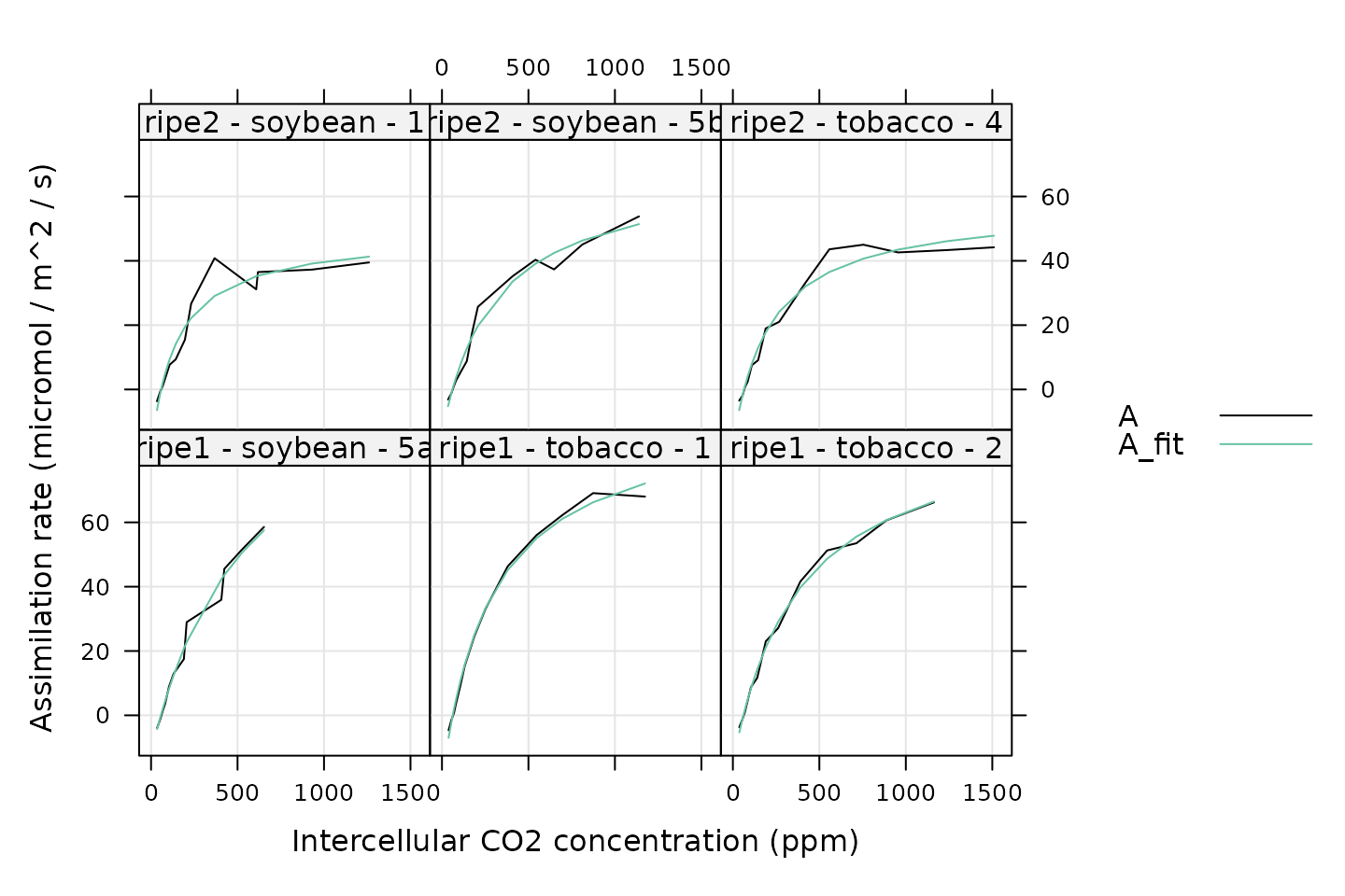
# Plot each fit
xyplot(
  A + A_fit ~ Ci | curve_identifier,
  data = c3_aci_results$fits$main_data,
  type = 'l',
  auto.key = list(space = 'right'),
  grid = TRUE,
  xlab = 'Intercellular CO2 concentration (ppm)',
  ylab = 'Assimilation rate (micromol / m^2 / s)',
  par.settings = list(
    superpose.line = list(col = multi_curve_colors()),
    superpose.symbol = list(col = multi_curve_colors())
  )
)


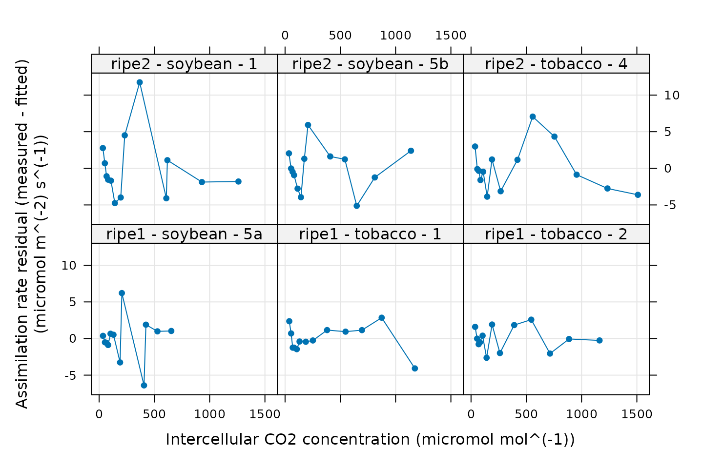
# Plot the residuals
xyplot(
  A_residuals ~ Ci | curve_identifier,
  data = c3_aci_results$fits$main_data,
  type = 'b',
  pch = 16,
  grid = TRUE,
  xlab = paste0('Intercellular CO2 concentration (',
    c3_aci_results$fits$units$Ci, ')'),
  ylab = paste0('Assimilation rate residual (measured - fitted)\n(',
    c3_aci_results$fits$units$A_residuals, ')')
)


# View the parameter values
columns_for_viewing <-
  c('instrument', 'species', 'plot', 'A_max', 'Ci_half', 'Rd', 'RMSE')

c3_aci_parameters <-
  c3_aci_results$parameters[ , columns_for_viewing, TRUE]

print(c3_aci_parameters)
#>   instrument [UserDefCon] (NA) species [UserDefCon] (NA) plot [UserDefCon] (NA)
#> 1                        ripe1                   soybean                     5a
#> 2                        ripe1                   tobacco                      1
#> 3                        ripe1                   tobacco                      2
#> 4                        ripe2                   soybean                      1
#> 5                        ripe2                   soybean                     5b
#> 6                        ripe2                   tobacco                      4
#>   A_max [fit_hyperbola] (micromol m^(-2) s^(-1))
#> 1                                      128.99658
#> 2                                      115.27665
#> 3                                      108.00753
#> 4                                       67.50371
#> 5                                       82.51852
#> 6                                       74.40790
#>   Ci_half [fit_hyperbola] (micromol mol^(-1))
#> 1                                    560.2505
#> 2                                    286.3507
#> 3                                    380.7208
#> 4                                    146.5151
#> 5                                    303.7394
#> 6                                    211.0452
#>   Rd [fit_hyperbola] (micromol m^(-2) s^(-1))
#> 1                                    11.89748
#> 2                                    20.57574
#> 3                                    14.89457
#> 4                                    19.17676
#> 5                                    13.73897
#> 6                                    17.46451
#>   RMSE [residual_stats] (micromol m^(-2) s^(-1))
#> 1                                       2.857247
#> 2                                       1.753694
#> 3                                       1.578398
#> 4                                       4.260341
#> 5                                       2.815101
#> 6                                       3.040083

More Examples

Another example can be found in the Combining PhotoGEA With Other Packages vignette, which discusses how to write wrappers for functions from other packages. Essentially, this is a specialized case of the ideas discussed here in this vignette.

Additional examples can be found by accessing the source code for the built-in processing functions provided with PhotoGEA. One way to see the code is to simply type the name of a function in the R terminal; for example, fit_ball_berry. Although this method is convenient, the downside is that any comments in the original code will not be included. An alternate way is to view the code on GitHub, where all the comments will be retained. For example, the source code for fit_ball_berry can be found by accessing the PhotoGEA GitHub page and navigating to R/fit_ball_berry.R.

Commands From This Document

The following code chunk includes all the central commands used throughout this document. They are compiled here to make them easy to copy/paste into a text file to initialize your own script.

# Load required packages
library(PhotoGEA)
library(lattice)

# Define a vector of paths to the files we wish to load
file_paths <- c(
  PhotoGEA_example_file_path('c3_aci_1.xlsx'),
  PhotoGEA_example_file_path('c3_aci_2.xlsx')
)

# Load each file, storing the result in a list
licor_exdf_list <- lapply(file_paths, function(fpath) {
  read_gasex_file(fpath, 'time')
})

# Get the names of all columns that are present in all of the Licor files
columns_to_keep <- do.call(identify_common_columns, licor_exdf_list)

# Extract just these columns
licor_exdf_list <- lapply(licor_exdf_list, function(x) {
  x[ , columns_to_keep, TRUE]
})

# Use `rbind` to combine all the data
licor_data <- do.call(rbind, licor_exdf_list)

# Create a new identifier column formatted like `instrument - species - plot`
licor_data[ , 'curve_identifier'] <-
  paste(licor_data[ , 'instrument'], '-', licor_data[ , 'species'], '-', licor_data[ , 'plot'])

# Make sure the data meets basic requirements
check_response_curve_data(licor_data, 'curve_identifier', 16, 'CO2_r_sp')

# Remove points with duplicated `CO2_r_sp` values and order by `Ci`
licor_data <- organize_response_curve_data(
    licor_data,
    'curve_identifier',
    c(9, 10),
    'Ci'
)

# Only keep points where stability was achieved
licor_data <- licor_data[licor_data[, 'Stable'] == 2, , TRUE]

# Remove any curves that have fewer than three remaining points
npts <- by(licor_data, licor_data[, 'curve_identifier'], nrow)
ids_to_keep <- names(npts[npts > 2])
licor_data <- licor_data[licor_data[, 'curve_identifier'] %in% ids_to_keep, , TRUE]

# Remove points where `instrument` is `ripe1` and `CO2_r_sp` is 1800
licor_data <- remove_points(
  licor_data,
  list(instrument = 'ripe1', CO2_r_sp = 1800)
)

# Define a custom fitting function
fit_hyperbola <- function(
  replicate_exdf,
  a_column_name = 'A',
  ci_column_name = 'Ci',
  initial_guess = list(A_max = 40, Ci_half = 100, Rd = 1)
)
{
  ### Check inputs

  if (!is.exdf(replicate_exdf)) {
      stop("fit_hyperbola requires an exdf object")
  }

  # Make sure the required variables are defined and have the correct units
  required_variables <- list()
  required_variables[[a_column_name]] <- "micromol m^(-2) s^(-1)"
  required_variables[[ci_column_name]] <- "micromol mol^(-1)"

  check_required_variables(replicate_exdf, required_variables)

  # Extract the values of several important columns
  A <- replicate_exdf[, a_column_name]
  Ci <- replicate_exdf[, ci_column_name]

  ### Perform processing operations

  # Wrap `stats::nls` in a `tryCatch` block so we can indicate fit failures by
  # setting `aci_fit` to `NULL`.
  aci_fit <- tryCatch(
    {
      stats::nls(A ~ A_max * Ci / (Ci + Ci_half) - Rd, start = initial_guess)
    },
    error = function(cond) {
      print('Having trouble fitting an A-Ci curve:')
      print(identifier_columns(replicate_exdf))
      print('Giving up on the fit :(')
      print(cond)
      return(NULL)
    },
    warning = function(cond) {
      print('Having trouble fitting an A-Ci curve:')
      print(identifier_columns(replicate_exdf))
      print('Giving up on the fit :(')
      print(cond)
      return(NULL)
    }
  )

  ### Collect and document outputs

  # Extract the fit results and add the fits and residuals to the exdf object
    if (is.null(aci_fit)) {
        A_max <- NA
        A_max_err <- NA
        Ci_half <- NA
        Ci_half_err <- NA
        Rd <- NA
        Rd_err <- NA
        replicate_exdf[, paste0(a_column_name, '_fit')] <- NA
        replicate_exdf[, paste0(a_column_name, '_residuals')] <- NA
    } else {
        fit_summary <- summary(aci_fit)
        A_max <- fit_summary$coefficients[1,1]
        A_max_err <- fit_summary$coefficients[1,2]
        Ci_half <- fit_summary$coefficients[2,1]
        Ci_half_err <- fit_summary$coefficients[2,2]
        Rd <- fit_summary$coefficients[3,1]
        Rd_err <- fit_summary$coefficients[3,2]

        replicate_exdf[, paste0(a_column_name, '_fit')] <-
          A_max * Ci / (Ci + Ci_half) - Rd

        replicate_exdf[, paste0(a_column_name, '_residuals')] <-
          fit_summary$residuals
    }

    # Document the columns that were added to the replicate exdf
    replicate_exdf <- document_variables(
        replicate_exdf,
        c('fit_hyperbola', paste0(a_column_name, '_fit'),       'micromol m^(-2) s^(-1)'),
        c('fit_hyperbola', paste0(a_column_name, '_residuals'), 'micromol m^(-2) s^(-1)')
    )

    # Get the replicate identifier columns
    replicate_identifiers <- identifier_columns(replicate_exdf)

    # Attach the residual stats to the identifiers
    replicate_identifiers <- cbind(
        replicate_identifiers,
        residual_stats(
            replicate_exdf[, paste0(a_column_name, '_residuals')],
            replicate_exdf$units[[a_column_name]],
            3
        )
    )

    # Add the values of the fitted parameters
    replicate_identifiers[, 'A_max'] <- A_max
    replicate_identifiers[, 'A_max_err'] <- A_max_err
    replicate_identifiers[, 'Ci_half'] <- Ci_half
    replicate_identifiers[, 'Ci_half_err'] <- Ci_half_err
    replicate_identifiers[, 'Rd'] <- Rd
    replicate_identifiers[, 'Rd_err'] <- Rd_err

    # Document the columns that were added
    replicate_identifiers <- document_variables(
        replicate_identifiers,
        c('fit_hyperbola', 'A_max',       'micromol m^(-2) s^(-1)'),
        c('fit_hyperbola', 'A_max_err',   'micromol m^(-2) s^(-1)'),
        c('fit_hyperbola', 'Ci_half',     'micromol mol^(-1)'),
        c('fit_hyperbola', 'Ci_half_err', 'micromol mol^(-1)'),
        c('fit_hyperbola', 'Rd',          'micromol m^(-2) s^(-1)'),
        c('fit_hyperbola', 'Rd_err',      'micromol m^(-2) s^(-1)')
    )

    return(list(
      fits = replicate_exdf,
      parameters = replicate_identifiers
    ))
}

# Fit each curve
c3_aci_results <- consolidate(by(
  licor_data,                       # The `exdf` object containing the curves
  licor_data[, 'curve_identifier'], # A factor used to split `licor_data` into chunks
  fit_hyperbola                     # The function to apply to each chunk of `licor_data`
))

# Plot each fit
xyplot(
  A + A_fit ~ Ci | curve_identifier,
  data = c3_aci_results$fits$main_data,
  type = 'l',
  auto.key = list(space = 'right'),
  grid = TRUE,
  xlab = 'Intercellular CO2 concentration (ppm)',
  ylab = 'Assimilation rate (micromol / m^2 / s)',
  par.settings = list(
    superpose.line = list(col = multi_curve_colors()),
    superpose.symbol = list(col = multi_curve_colors())
  )
)

# Plot the residuals
xyplot(
  A_residuals ~ Ci | curve_identifier,
  data = c3_aci_results$fits$main_data,
  type = 'b',
  pch = 16,
  grid = TRUE,
  xlab = paste0('Intercellular CO2 concentration (',
    c3_aci_results$fits$units$Ci, ')'),
  ylab = paste0('Assimilation rate residual (measured - fitted)\n(',
    c3_aci_results$fits$units$A_residuals, ')')
)

# View the parameter values
columns_for_viewing <-
  c('instrument', 'species', 'plot', 'A_max', 'Ci_half', 'Rd', 'RMSE')

c3_aci_parameters <-
  c3_aci_results$parameters[ , columns_for_viewing, TRUE]

print(c3_aci_parameters)