Calculate Rd using the Laisk method — calculate_rd

Uses the Laisk method to estimate CiStar and Rd. This function can accomodate alternative colum names for the variables taken from log files in case they change at some point in the future. This function also checks the units of each required column and will produce an error if any units are incorrect.

Usage

calculate_rd_laisk(
    exdf_obj,
    curve_id_column_name,
    ci_lower = 40,
    ci_upper = 120,
    a_column_name = 'A',
    ci_column_name = 'Ci'
  )

Arguments

exdf_obj: An exdf object.
curve_id_column_name: The name of the column in exdf_obj that can be used to split it into individual response curves.
ci_lower: Lower end of Ci range used for linear fits of An vs. Ci.
ci_upper: Upper end of Ci range used for linear fits of An vs. Ci.
a_column_name: The name of the column in exdf_obj that contains the net CO2 assimilation rate An in micromol m^(-2) s^(-1).
ci_column_name: The name of the column in exdf_obj that contains the intercellular CO2 concentration Ci in micromol mol^(-1).

Details

The Laisk method is a way to estimate Rd and CiStar for a C3 plant. Definitions of these quantities and a description of the theory underpinning this method is given below.

For a C3 plant, the net CO2 assimilation rate An is given by

An = Vc - Rp - Rd,

where Vc is the rate of RuBP carboxylation, Rp is the rate of carbon loss due to photorespiration, and Rd is the rate of carbon loss due to non-photorespiratory respiration (also known as the rate of day respiration). Because RuBP carboxylation and photorespiration both occur due to Rubisco activity, these rates are actually proportional to each other:

Rp = Vc * GammaStar / Cc,

where Cc is the CO2 concentration in the chloroplast (where Rubisco is located) and GammaStar will be discussed below. Using this expression, the net CO2 assimilation rate can be written as

An = Vc * (1 - GammaStar / Cc) - Rd.

When Cc is equal to GammaStar, the net assimilation rate is equal to -Rd. For this reason, GammaStar is usually referred to as the CO2 compensation point in the absence of day respiration.

In general, Cc is related to the intercellular CO2 concentration Ci according to

Ci = Cc + An / gmc,

where gmc is the mesophyll conductance to CO2 diffusion. When Cc is equal to GammaStar, we therefore have Ci = GammaStar - Rd / gmc. This special value of Ci is referred to as CiStar, and can be understood as the value of Ci where Cc = GammaStar and An = -Rd. Note that the values of GammaStar and CiStar depend on Rubisco properties, mesophyll conductance, and the ambient O2 concentration, but not on the incident light intensity.

These observations suggest a method for estimating Rd from a leaf: Measure An vs. Ci curves at several light intensities, and find the value of Ci where the curves intersect with each other. This will be CiStar, and the corresponding value of An will be equal to -Rd.

In practice, it is unlikely that the measured curves will all exactly intersect at a single point. In calculate_rd_laisk, the value of CiStar is chosen as the value of Ci that minimizes the variance of the corresponding An values. It is also unlikely that any of the measured points exactly correspond to Ci = CiStar, so calculate_rd_laisk uses a linear fit of each curve at low Ci to find An at arbitrary values of Ci.

Note: it is possible that Rd depends on incident light intensity, an issue which complicates the application of the Laisk method.

References:

Yin, X., Sun, Z., Struik, P. C. & Gu, J. "Evaluating a new method to estimate the rate of leaf respiration in the light by analysis of combined gas exchange and chlorophyll fluorescence measurements." Journal of Experimental Botany 62, 3489–3499 (2011) [doi:10.1093/jxb/err038 ].

Value

This function returns a list with the following named elements:

Ci_star: The estimated value of CiStar.
Rd: The estimated value of Rd.
parameters: An exdf object with the slope and intercept of each linear fit used to estimate Ci_star and Rd.
fits: An exdf object based on exdf_obj that also includes the fitted values of An in a new column whose name is a_column_name followed by _fit (for example, A_fit).

Examples

# Read an example Licor file included in the PhotoGEA package
licor_file <- read_gasex_file(
  PhotoGEA_example_file_path('c3_aci_1.xlsx')
)

# Define a new column that uniquely identifies each curve
licor_file[, 'species_plot'] <-
  paste(licor_file[, 'species'], '-', licor_file[, 'plot'] )

# Organize the data
licor_file <- organize_response_curve_data(
    licor_file,
    'species_plot',
    c(9, 10, 16),
    'CO2_r_sp'
)

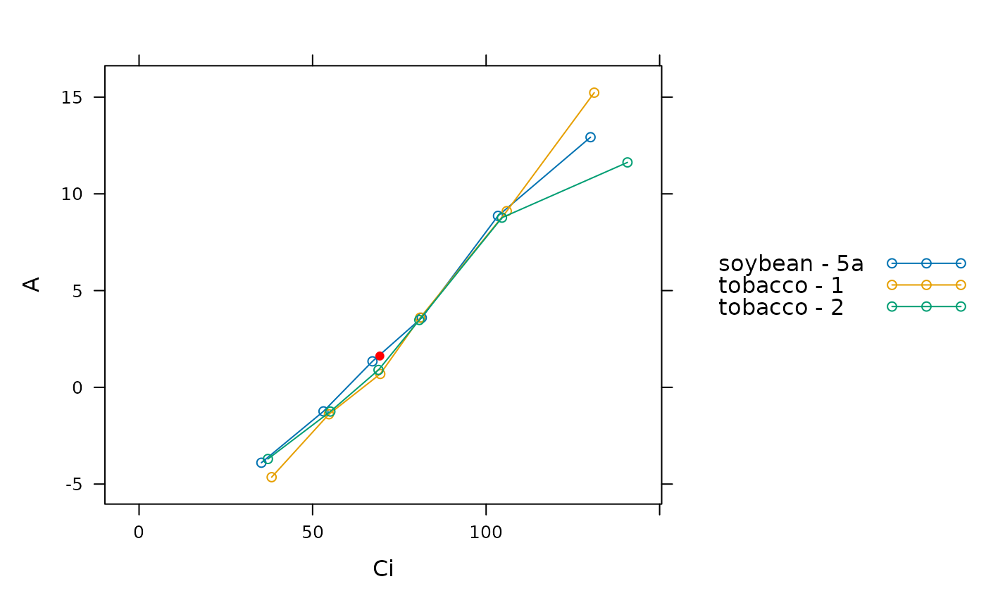
# Apply the Laisk method. Note: this is a bad example because these curves were
# measured at the same light intensity, but from different species. Because of
# this, the results are not meaningful.
laisk_results <- calculate_rd_laisk(licor_file, 'species_plot', 20, 150)

# Get estimated values
print(laisk_results$Rd)
#> [1] -1.617453
print(laisk_results$Ci_star)
#> [1] 69.37657

# Plot each curve and overlay the calculated point of intersection as a filled
# red circle
lattice::xyplot(
  A ~ Ci,
  group = species_plot,
  data = laisk_results$fits$main_data,
  type = 'b',
  auto = TRUE,
  panel = function(...) {
      lattice::panel.xyplot(...)
      lattice::panel.points(
          -laisk_results$Rd ~ laisk_results$Ci_star,
          type = 'p',
          col = 'red',
          pch = 16
      )
  }
)


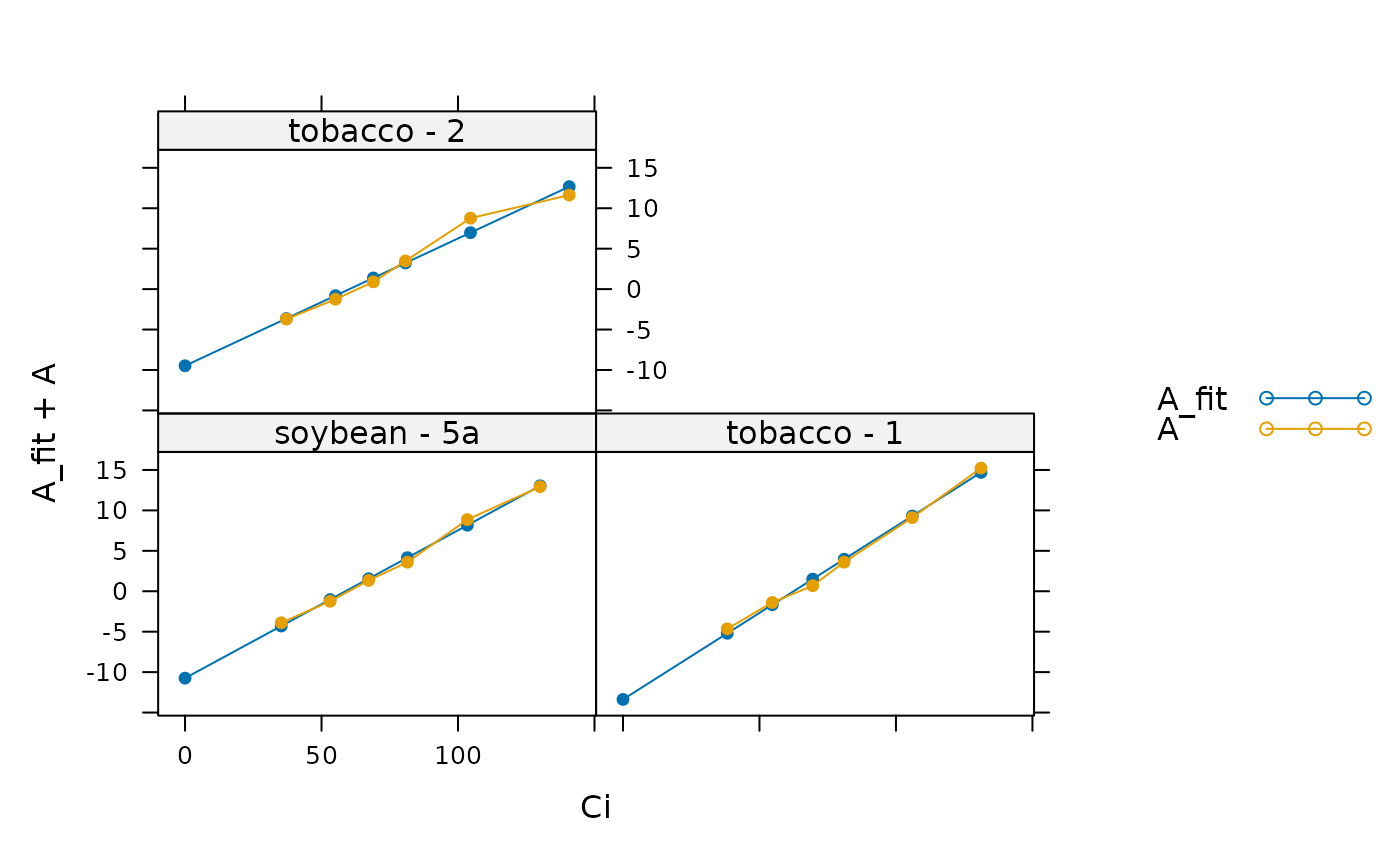
# Plot each curve and its linear fit
lattice::xyplot(
  A_fit + A ~ Ci | species_plot,
  data = laisk_results$fits$main_data,
  type = 'b',
  pch = 16,
  auto = TRUE
)