Fits a C4 assimilation model to an experimental curve

Fits a model to an experimentally measured C4 CO2 response curve using the data in the exdf object along with a few other user-supplied parameters. This function can accomodate alternative column names for the variables taken from the Licor file in case they change at some point in the future. This function also checks the units of each required column and will produce an error if any units are incorrect.

Usage

fit_c4_aci(
    replicate_exdf,
    Ca_atmospheric = NA,
    ao_column_name = 'ao',
    a_column_name = 'A',
    ca_column_name = 'Ca',
    ci_column_name = 'Ci',
    gamma_star_column_name = 'gamma_star',
    jmax_norm_column_name = 'Jmax_norm',
    kc_column_name = 'Kc',
    ko_column_name = 'Ko',
    kp_column_name = 'Kp',
    oxygen_column_name = 'oxygen',
    pcm_column_name = 'PCm',
    qin_column_name = 'Qin',
    rl_norm_column_name = 'RL_norm',
    total_pressure_column_name = 'total_pressure',
    vcmax_norm_column_name = 'Vcmax_norm',
    vpmax_norm_column_name = 'Vpmax_norm',
    sd_A = 'RMSE',
    absorptance = 0.85,
    f_spectral = 0.15,
    rho = 0.5,
    theta = 0.7,
    x_etr = 0.4,
    OPTIM_FUN = optimizer_deoptim(200),
    lower = list(),
    upper = list(),
    fit_options = list(),
    error_threshold_factor = 0.147,
    hard_constraints = 0,
    calculate_confidence_intervals = TRUE,
    remove_unreliable_param = 2
  )

Arguments

replicate_exdf: An exdf object representing one CO2 response curve.
Ca_atmospheric: The atmospheric CO2 concentration (with units of micromol mol^(-1)); this will be used by estimate_operating_point to estimate the operating point. A value of NA disables this feature.
ao_column_name: The name of the column in exdf_obj that contains the dimensionless ratio of solubility and diffusivity of O2 to CO2.
a_column_name: The name of the column in replicate_exdf that contains the net assimilation in micromol m^(-2) s^(-1).
ca_column_name: The name of the column in replicate_exdf that contains the ambient CO2 concentration in micromol mol^(-1).
ci_column_name: The name of the column in replicate_exdf that contains the intercellular CO2 concentration in micromol mol^(-1).
gamma_star_column_name: The name of the column in exdf_obj that contains the dimensionless gamma_star values.
jmax_norm_column_name: The name of the column in exdf_obj that contains the normalized Jmax values (with units of normalized to Jmax at its optimal temperature).
kc_column_name: The name of the column in exdf_obj that contains the Michaelis-Menten constant for rubisco carboxylation in microbar.
ko_column_name: The name of the column in exdf_obj that contains the Michaelis-Menten constant for rubisco oxygenation in mbar.
kp_column_name: The name of the column in exdf_obj that contains the Michaelis-Menten constant for PEP carboxylase carboxylation in microbar.
oxygen_column_name: The name of the column in exdf_obj that contains the concentration of O2 in the ambient air, expressed as a percentage (commonly 21% or 2%); the units must be percent.
pcm_column_name: The name of the column in exdf_obj that contains the partial pressure of CO2 in the mesophyll, expressed in microbar.
qin_column_name: The name of the column in exdf_obj that contains values of the incident photosynthetically active flux density in micromol m^(-2) s^(-1).
rl_norm_column_name: The name of the column in exdf_obj that contains the normalized RL values (with units of normalized to RL at 25 degrees C).
total_pressure_column_name: The name of the column in exdf_obj that contains the total pressure in bar.
vcmax_norm_column_name: The name of the column in exdf_obj that contains the normalized Vcmax values (with units of normalized to Vcmax at 25 degrees C).
vpmax_norm_column_name: The name of the column in exdf_obj that contains the normalized Vpmax values (with units of normalized to Vpmax at 25 degrees C).
sd_A: A value of the standard deviation of measured A values, or the name of a method for determining the deviation; currently, the only supported option is 'RMSE'.
absorptance: The leaf absorptance (dimensionless). See Equation 35 from S. von Caemmerer (2021).
f_spectral: The spectral quality adjustment factor (dimensionless). See Equation 35 from S. von Caemmerer (2021).
rho: The fraction of light absorbed by photosystem II rather than photosystem I (dimensionless). See Equation 35 from S. von Caemmerer (2021).
theta: An empirical curvature factor (dimensionless). See Equation 34 from S. von Caemmerer (2021).
x_etr: The fraction of whole-chain electron transport occurring in the mesophyll (dimensionless). See Equation 29 from S. von Caemmerer (2021).
OPTIM_FUN: An optimization function that accepts the following input arguments: an initial guess, an error function, lower bounds, and upper bounds. It should return a list with the following elements: par, convergence, value, and (optionally) message. See optimizers for a list of available options.
lower: A list of named numeric elements representing lower bounds to use when fitting. Values supplied here override the default values (see details below). For example, lower = list(Vcmax_at_25 = 10) sets the lower limit for Vcmax_at_25 to 10 micromol / m^2 / s.
upper: A list of named numeric elements representing upper bounds to use when fitting. Values supplied here override the default values (see details below). For example, upper = list(Vcmax_at_25 = 200) sets the upper limit for Vcmax_at_25 to 200 micromol / m^2 / s.
fit_options: A list of named elements representing fit options to use for each parameter. Values supplied here override the default values (see details below). Each element must be 'fit', 'column', or a numeric value. A value of 'fit' means that the parameter will be fit; a value of 'column' means that the value of the parameter will be taken from a column in exdf_obj of the same name; and a numeric value means that the parameter will be set to that value. For example, fit_options = list(RL_at_25 = 0, Vcmax_at_25 = 'fit', Vpr = 'column') means that RL_at_25 will be set to 0, Vcmax_at_25 will be fit, and Vpr will be set to the values in the Vpr column of exdf_obj.
error_threshold_factor: To be passed to confidence_intervals_c4_aci when calculate_confidence_intervals is TRUE.
hard_constraints: To be passed to calculate_c4_assimilation; see that function for more details.
calculate_confidence_intervals: A logical value indicating whether or not to estimate confidence intervals for the fitting parameters using confidence_intervals_c4_aci.
remove_unreliable_param: An integer value indicating the rules to use when identifying and removing unreliable parameter estimates. A value of 2 is the most conservative option. A value of 0 disables this feature, which is not typically recommended. See below for more details.

Details

This function calls calculate_c4_assimilation to calculate values of net assimilation. The user-supplied optimization function is used to vary the values of alpha_psii, gbs, Jmax_at_opt, RL_at_25, Rm_frac, Vcmax_at_25, Vpmax_at_25, and Vpr to find ones that best reproduce the experimentally measured values of net assimilation. By default, the following options are used for the fits:

alpha_psii: lower = -1, upper = 10, fit_option = 0
gbs: lower = -1, upper = 10, fit_option = 0.003
Jmax_at_opt: lower = -50, upper = 1000, fit_option = 1000
RL_at_25: lower = -10, upper = 100, fit_option = 'fit'
Rm_frac: lower = -10, upper = 10, fit_option = 0.5
Vcmax_at_25: lower = -50, upper = 1000, fit_option = 'fit'
Vpmax_at_25: lower = -50, upper = 1000, fit_option = 'fit'
Vpr: lower = -50, upper = 1000, fit_option = 1000

With these settings, Jmax and Vpr are set to 1000 (so net assimilation is essentially never limited by light or PEP carboxylase regeneration), alpha_psii, gbs, and Rm_frac are set to default values used in von Caemmerer (2000), and the other parameters are fit during the process (see fit_options above). The bounds are chosen liberally to avoid any bias.

An initial guess for the parameters is generated by calling initial_guess_c4_aci with the pcm_threshold_rlm argument set to 40 microbar. Note that any fixed values specified in the fit options will override the values returned by the guessing function.

The fit is made by creating an error function using error_function_c4_aci and minimizing its value using OPTIM_FUN, starting from the initial guess described above. The optimizer_deoptim optimizer is used by default since it has been found to reliably return great fits. However, it is a slow optimizer. If speed is important, consider reducing the number of generations or using optimizer_nmkb, but be aware that this optimizer is more likely to get stuck in a local minimum.

The photosynthesis model represented by calculate_c4_assimilation is not smooth in the sense that small changes in the input parameters do not necessarily cause changes in its outputs. This is related to the calculation of the PEP carboxylase activity Vp, which is taken to be the minimum of Vpr and Vpc. For example, if Vpr is high and Vp = Vpc at all points along the curve, modifying Vpr by a small amount will not change the model's outputs. Similar issues can occur when calculating An as the minimum of Ac and Aj. Because of this, derivative-based optimizers tend to struggle when fitting C4 A-Ci curves. Best results are obtained using derivative-free methods. It has been found that dfoptim::nmkb is often able to find a good fit.

Sometimes the optimizer may choose a set of parameter values where one of the potential limiting rates Vpc or Vpr is never the smallest rate. In this case, the corresponding parameter estimates (Vpmax or Vpr) will be unreliable. Likewise, it may happen that one of Ac or Aj is never the smallest rate. In this case the corresponding parameter estimates (Vpmax, Vpr, and Vcmax, or Jmax) will be unreliable. If remove_unreliable_param is 1 or larger, then such parameter estimates (and the corresponding rates) will be replaced by NA in the fitting results.

It is also possible that the upper limit of the confidence interval for a parameter is infinity; this also indicates an unreliable parameter estimate. If remove_unreliable_param is 2 or larger, then such parameter estimates (but not the corresponding rates) will be replaced by NA in the fitting results.

These criteria are used to determine the reliability of each parameter estimate, which is indicated in the Vpmax_trust, Vpr_trust, and Vcmax_trust columns of the output from fit_c4_aci, where a value of 0 indicates an unreliable estimate and 1 indicates a reliable estimate.

Once the best-fit parameters have been determined, this function also estimates the operating value of `PCm from the atmospheric CO2 concentration atmospheric_ca using estimate_operating_point, and then uses that value to estimate the modeled An at the operating point via calculate_c4_assimilation. It also estimates the Akaike information criterion (AIC).

This function assumes that replicate_exdf represents a single C4 A-Ci curve. To fit multiple curves at once, this function is often used along with by.exdf and consolidate.

Value

A list with two elements:

fits: An exdf object including the original contents of replicate_exdf along with several new columns:
- The fitted values of net assimilation will be stored in a column whose name is determined by appending '_fit' to the end of a_column_name; typically, this will be 'A_fit'.
- Residuals (measured - fitted) will be stored in a column whose name is determined by appending '_residuals' to the end of a_column_name; typically, this will be 'A_residuals'.
- Values of fitting parameters at 25 degrees C (or the optimal temperature) will be stored in the Jmax_at_opt, RL_at_25, Vcmax_at_25, Vpmax_at_25, and Vpr columns.
- The other outputs from calculate_c4_assimilation will be stored in columns with the usual names: alpha_psii, gbs, Rm_Frac, Vcmax_tl, Vpmax_tl, RL_tl, RLm_tl, Vp, Apc, Apr, Ap, Ar, Ajm, Ajbs, Ac, and Aj.
fits_interpolated: An exdf object including the calculated assimilation rates at a fine spacing of Ci values (step size of 1 micromol mol^(-1)).
parameters: An exdf object including the identifiers, fitting parameters, and convergence information for the A-Ci curve:
- The number of points where Vpc and Vpr are each the smallest potential carboxylation rate are stored in the n_Vpc_smallest and n_Vpr_smallest columns.
- The best-fit values are stored in the alpha_psii, gbs, Jmax_at_opt RL_at_25, Rm_frac, Vcmax_at_25, Vpmax_at_25, and Vpr columns. If calculate_confidence_intervals is TRUE, upper and lower limits for each of these parameters will also be included.
- For parameters that depend on leaf temperature, the average leaf-temperature-dependent values are stored in X_tl_avg columns: J_tl_avg, Jmax_tl_avg, RL_tl_avg, Vcmax_tl_avg, and Vpmax_tl_avg.
- Information about the operating point is stored in operating_PCm, operating_Ci, operating_An, and operating_An_model.
- The convergence column indicates whether the fit was successful (==0) or if the optimizer encountered a problem (!=0).
- The feval column indicates how many cost function evaluations were required while finding the optimal parameter values.
- The residual stats as returned by residual_stats are included as columns with the default names: dof, RSS, RMSE, etc.
- The Akaike information criterion is included in the AIC column.

Examples

# Read an example Licor file included in the PhotoGEA package
licor_file <- read_gasex_file(
  PhotoGEA_example_file_path('c4_aci_1.xlsx')
)

# Define a new column that uniquely identifies each curve
licor_file[, 'species_plot'] <-
  paste(licor_file[, 'species'], '-', licor_file[, 'plot'] )

# Organize the data
licor_file <- organize_response_curve_data(
    licor_file,
    'species_plot',
    c(9, 10, 16),
    'CO2_r_sp'
)

# Calculate temperature-dependent values of C4 photosynthetic parameters
licor_file <- calculate_arrhenius(licor_file, c4_arrhenius_von_caemmerer)

licor_file <- calculate_peaked_gaussian(licor_file, c4_peaked_gaussian_von_caemmerer)

# Calculate the total pressure in the Licor chamber
licor_file <- calculate_total_pressure(licor_file)

# Calculate PCm
licor_file <- apply_gm(licor_file, 'C4')

# For these examples, we will use a faster (but sometimes less reliable)
# optimizer so they run faster
optimizer <- optimizer_nmkb(1e-7)

# Fit just one curve from the data set (it is rare to do this).
one_result <- fit_c4_aci(
  licor_file[licor_file[, 'species_plot'] == 'maize - 5', , TRUE],
  Ca_atmospheric = 420,
  OPTIM_FUN = optimizer
)

# Fit all curves in the data set (it is more common to do this)
aci_results <- consolidate(by(
  licor_file,
  licor_file[, 'species_plot'],
  fit_c4_aci,
  Ca_atmospheric = 420,
  OPTIM_FUN = optimizer
))

# View the fitting parameters for each species / plot
col_to_keep <- c(
  'species', 'plot',                                       # identifiers
  'RL_at_25', 'Vcmax_at_25', 'Vpmax_at_25', 'Vpr',         # parameters scaled to 25 degrees C
  'RL_tl_avg', 'Vcmax_tl_avg', 'Vpmax_tl_avg',             # average temperature-dependent values
  'operating_Ci', 'operating_An', 'operating_An_model',    # operating point info
  'dof', 'RSS', 'MSE', 'RMSE', 'RSE',                      # residual stats
  'convergence', 'convergence_msg', 'feval', 'optimum_val' # convergence info
)

aci_results$parameters[ , col_to_keep, TRUE]
#>   species [UserDefCon] (NA) plot [UserDefCon] (NA)
#> 1                     maize                      5
#> 2                   sorghum                      2
#> 3                   sorghum                      3
#>   RL_at_25 [fit_c4_aci] (micromol m^(-2) s^(-1))
#> 1                                     -2.9754811
#> 2                                      0.7308282
#> 3                                     -3.8073918
#>   Vcmax_at_25 [fit_c4_aci] (micromol m^(-2) s^(-1))
#> 1                                          33.90720
#> 2                                          42.62026
#> 3                                          35.99262
#>   Vpmax_at_25 [fit_c4_aci] (micromol m^(-2) s^(-1))
#> 1                                          158.2056
#> 2                                          149.4451
#> 3                                          124.2471
#>   Vpr [fit_c4_aci] (micromol m^(-2) s^(-1))
#> 1                                        NA
#> 2                                        NA
#> 3                                        NA
#>   RL_tl_avg [fit_c4_aci] (micromol m^(-2) s^(-1))
#> 1                                       -4.754837
#> 2                                        1.132770
#> 3                                       -6.101126
#>   Vcmax_tl_avg [fit_c4_aci] (micromol m^(-2) s^(-1))
#> 1                                           58.81068
#> 2                                           71.31746
#> 3                                           62.63551
#>   Vpmax_tl_avg [fit_c4_aci] (micromol m^(-2) s^(-1))
#> 1                                           225.3235
#> 2                                           208.0097
#> 3                                           177.3184
#>   operating_Ci [estimate_operating_point] (micromol mol^(-1))
#> 1                                                    183.4839
#> 2                                                    166.2077
#> 3                                                    158.8843
#>   operating_An [estimate_operating_point] (micromol m^(-2) s^(-1))
#> 1                                                         52.35755
#> 2                                                         51.85285
#> 3                                                         51.32954
#>   operating_An_model [fit_c4_aci] (micromol m^(-2) s^(-1))
#> 1                                                 56.49677
#> 2                                                 58.59113
#> 3                                                 56.40293
#>   dof [residual_stats] (NA) RSS [residual_stats] ((micromol m^(-2) s^(-1))^2)
#> 1                        10                                         217.81625
#> 2                        10                                         448.94801
#> 3                        10                                          48.82484
#>   MSE [residual_stats] ((micromol m^(-2) s^(-1))^2)
#> 1                                         16.755096
#> 2                                         34.534462
#> 3                                          3.755757
#>   RMSE [residual_stats] (micromol m^(-2) s^(-1))
#> 1                                       4.093299
#> 2                                       5.876603
#> 3                                       1.937978
#>   RSE [residual_stats] (micromol m^(-2) s^(-1)) convergence [fit_c4_aci] ()
#> 1                                      4.667079                           0
#> 2                                      6.700358                           0
#> 3                                      2.209634                           0
#>   convergence_msg [fit_c4_aci] () feval [fit_c4_aci] ()
#> 1          Successful convergence                   150
#> 2          Successful convergence                   209
#> 3          Successful convergence                   162
#>   optimum_val [fit_c4_aci] ()
#> 1                    36.76777
#> 2                    41.46893
#> 3                    27.04758

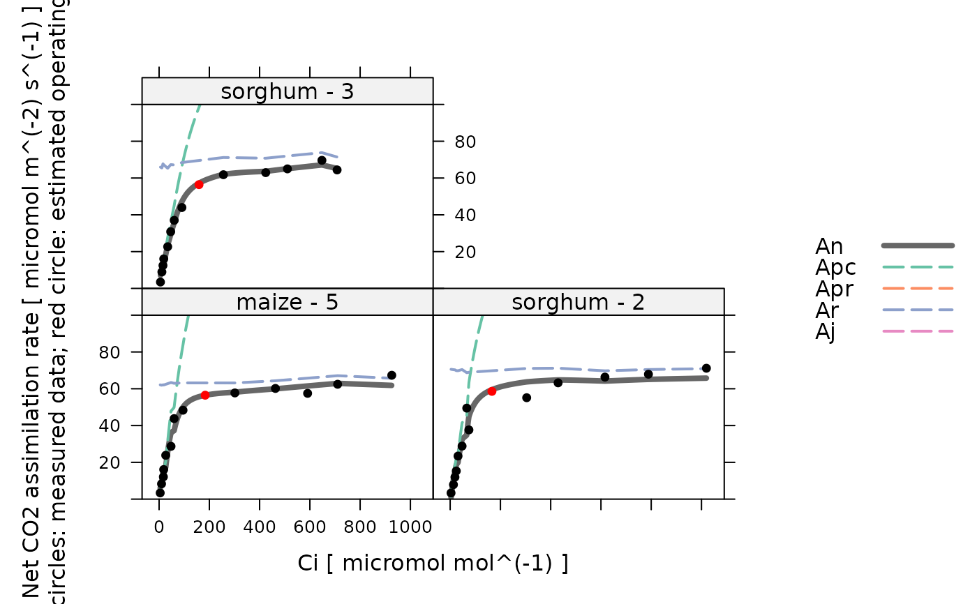
# View the fits for each species / plot
plot_c4_aci_fit(aci_results, 'species_plot', 'Ci', ylim = c(0, 100))


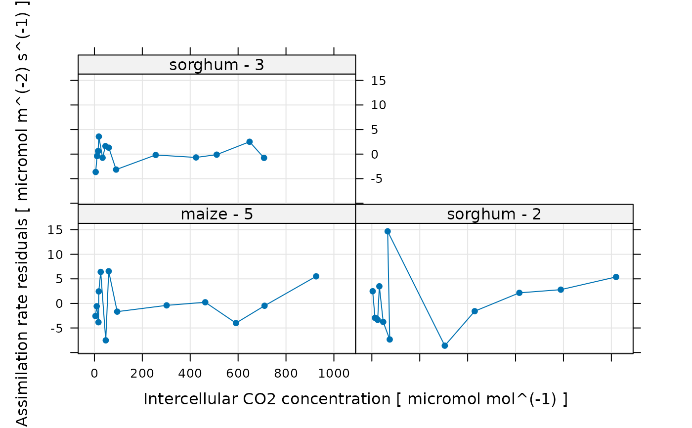
# View the residuals for each species / plot
lattice::xyplot(
  A_residuals ~ Ci | species_plot,
  data = aci_results$fits$main_data,
  type = 'b',
  pch = 16,
  auto = TRUE,
  grid = TRUE,
  xlab = paste('Intercellular CO2 concentration [', aci_results$fits$units$Ci, ']'),
  ylab = paste('Assimilation rate residuals [', aci_results$fits$units$A_residuals, ']')
)