Make an initial guess of C4 photosynthesis parameter values for one curve

Creates a function that makes an initial guess of C4 photosynthesis model parameter values for one curve. This function is used internally by fit_c4_aci.

Values estimated by this guessing function should be considered inaccurate, and should always be improved upon by an optimizer.

Usage

initial_guess_c4_aci(
    alpha_psii,
    gbs,
    Rm_frac,
    pcm_threshold_rlm = 40,
    absorptance = 0.85,
    f_spectral = 0.15,
    rho = 0.5,
    theta = 0.7,
    x_etr = 0.4,
    a_column_name = 'A',
    jmax_norm_column_name = 'Jmax_norm',
    kp_column_name = 'Kp',
    pcm_column_name = 'PCm',
    qin_column_name = 'Qin',
    rl_norm_column_name = 'RL_norm',
    vcmax_norm_column_name = 'Vcmax_norm',
    vpmax_norm_column_name = 'Vpmax_norm'
  )

Arguments

alpha_psii: The fraction of photosystem II activity in the bundle sheath (dimensionless). If alpha_psii is not a number, then there must be a column in exdf_obj called alpha_psii with appropriate units. A numeric value supplied here will overwrite the values in the alpha_psii column of exdf_obj if it exists.
gbs: The bundle sheath conductance to CO2 in mol m^(-2) s^(-1) bar^(-1). If gbs is not a number, then there must be a column in exdf_obj called gbs with appropriate units. A numeric value supplied here will overwrite the values in the gbs column of exdf_obj if it exists.
Rm_frac: The fraction of the total mitochondrial respiration that occurs in the mesophyll. If Rm_frac is not a number, then there must be a column in exdf_obj called Rm_frac with appropriate units. A numeric value supplied here will overwrite the values in the Rm_frac column of exdf_obj if it exists.
pcm_threshold_rlm: An upper cutoff value for the partial pressure of CO2 in the mesophyll (in microbar) to be used when estimating RLm.
absorptance: The leaf absorptance (dimensionless). See Equation 35 from S. von Caemmerer (2021).
f_spectral: The spectral quality adjustment factor (dimensionless). See Equation 35 from S. von Caemmerer (2021).
rho: The fraction of light absorbed by photosystem II rather than photosystem I (dimensionless). See Equation 35 from S. von Caemmerer (2021).
theta: An empirical curvature factor (dimensionless). See Equation 34 from S. von Caemmerer (2021).
x_etr: The fraction of whole-chain electron transport occurring in the mesophyll (dimensionless). See Equation 29 from S. von Caemmerer (2021).
a_column_name: The name of the column in licor_exdf that contains the net assimilation in micromol m^(-2) s^(-1).
jmax_norm_column_name: The name of the column in exdf_obj that contains the normalized Jmax values (with units of normalized to Jmax at its optimal temperature).
kp_column_name: The name of the column in exdf_obj that contains the Michaelis-Menten constant for PEP carboxylase carboxylation in microbar.
pcm_column_name: The name of the column in exdf_obj that contains the partial pressure of CO2 in the mesophyll, expressed in microbar.
qin_column_name: The name of the column in exdf_obj that contains values of the incident photosynthetically active flux density in micromol m^(-2) s^(-1).
rl_norm_column_name: The name of the column in exdf_obj that contains the normalized RL values (with units of normalized to RL at 25 degrees C).
vcmax_norm_column_name: The name of the column in exdf_obj that contains the normalized Vcmax values (with units of normalized to Vcmax at 25 degrees C).
vpmax_norm_column_name: The name of the column in exdf_obj that contains the normalized Vpmax values (with units of normalized to Vpmax at 25 degrees C).

Details

Here we estimate values of Jmax_at_opt, RL_at_25, Vcmax_at_25, Vpmax_at_25, and Vpr from a measured C4 CO2 response curve. It is difficult to estimate values of alpha_psii, gbs, and Rm_frac from a curve, so they must be supplied beforehand. For more information about these parameters, see the documentation for calculate_c4_assimilation. To estimate these parameter values, we use several equations from S. von Caemmerer, "Biochemical Models of Leaf Photosynthesis" (CSIRO Publishing, 2000) [doi:10.1071/9780643103405 ]. Any equation numbers referenced below are from this book.

Estimating RL: An estimate for RLm can be obtained using Equation 4.26, which applies for low values of PCm. In this situation, PCm + Kp can be approximated by Kp, and Equation 4.26 simplifies to a linear relationship between the net assimilation An and PCm: An = (gbs + Vpmax / kP) * PCm - RLm. So, to estimate RLm, we make a linear fit of An vs. PCm in the low PCm range where this equation is expected to be valid. Then RLm is given by the negative of the intercept from the fit. In the C4 assimilation model, we assume that RLm = Rm_frac * RL, so we can also estimate RL = RLm / Rm_frac from this value.
Estimating Vpmax: An estimate for Vpmax can also be obtained from Equation 4.26. In this case, we simply solve the equation for Vpmax and use it to calculate a value of Vpmax at each point in the curve from the measured values of An and PCm, the input value of gbs, and the value of RLm estimated above. In the PEP-carboxylation-limited range, the estimated values of Vpmax should be reasonable. In other parts of the curve, the assimilation rate is limited by other factors, so An will be smaller than the PEP-carboxylation-limited values, causing the estimated values of Vpmax to be smaller. So, to make an overall estimate, we choose the largest estimated Vpmax value.
Estimating Vcmax: An estimate for Vcmax can be obtained by solving An = Vcmax - RL for Vcmax, similar to the method used to estimate Vpmax.
Estimating Vpr: An estimate for Vpr can be obtained by solving An = Vpr + gbs * PCm - RLm for Vpr, similar to the method used to estimate Vpmax.
Estimating Jmax: First, an estimate for J can be obtained by solving An = (1 - x_etr) * J / 3 - RL for J. Then, estimates of Jmax can be made from J and Qin. The largest value of Jmax / Jmax_norm is chosen as the best estimate for Jmax_at_opt.

Note that a key assumption underlying this approach is that the net assimilation can be reasonably approximated by An = min(Apc, Apr, Ar, Ajm) (Equations 4.19, 4.25, 4.45, and 4.47 combined). While this approximation seems to work well for low values of PCm, it tends to deviate significantly from the more accurate version at higher values of PCm, predicting values that are noticably smaller. Thus, the values of Vcmax and Vpr estimated using this procedure are unlikely to be accurate. This is not a problem; instead it simply highlights the importance of improving this initial guess using an optimizer, which can be accomplished via fit_c4_aci.

Value

A function with one input argument rc_exdf, which should be an exdf object representing one C4 CO2 response curve. The return value of this function will be a numeric vector with eight elements, representing the values of alpha_psii, gbs, Jmax_at_opt, RL_at_25, rm_frac, Vcmax_at_25, Vpmax_at_25, and Vpr (in that order).

Examples

# Read an example Licor file included in the PhotoGEA package
licor_file <- read_gasex_file(
  PhotoGEA_example_file_path('c4_aci_1.xlsx')
)

# Define a new column that uniquely identifies each curve
licor_file[, 'species_plot'] <-
  paste(licor_file[, 'species'], '-', licor_file[, 'plot'] )

# Organize the data
licor_file <- organize_response_curve_data(
    licor_file,
    'species_plot',
    c(9, 10, 16),
    'CO2_r_sp'
)

# Calculate temperature-dependent values of C4 photosynthetic parameters
licor_file <- calculate_arrhenius(licor_file, c4_arrhenius_von_caemmerer)

licor_file <- calculate_peaked_gaussian(licor_file, c4_peaked_gaussian_von_caemmerer)

# Calculate the total pressure in the Licor chamber
licor_file <- calculate_total_pressure(licor_file)

# Calculate PCm
licor_file <- apply_gm(licor_file, 'C4')

# Create the guessing function, using typical values for the alpha_psii, gbs,
# and Rm_frac: 0, 0.003, and 0.5
guessing_func <- initial_guess_c4_aci(0, 0.003, 0.5)

# Apply it and see the initial guesses for each curve
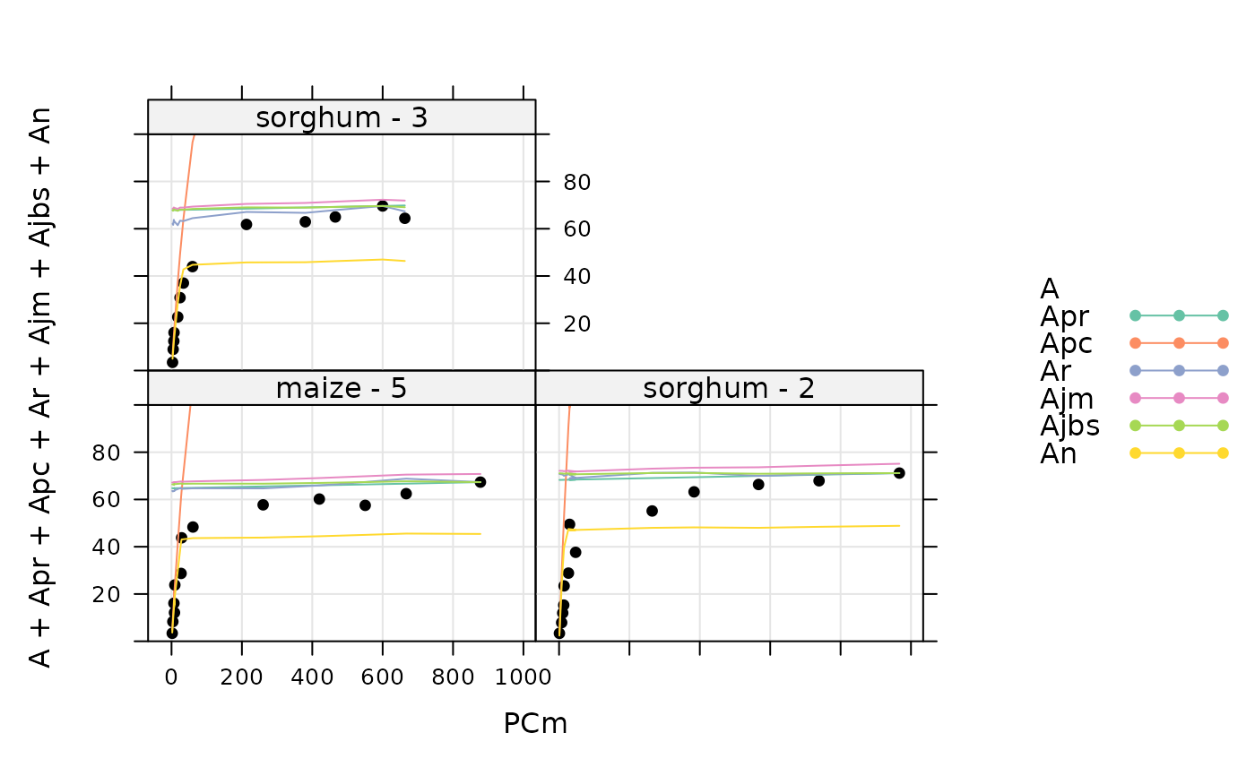
str(by(licor_file, licor_file[, 'species_plot'], guessing_func))
#> List of 3
#>  $ maize - 5  : num [1:8] 0 0.003 550.867 1 0.5 ...
#>  $ sorghum - 2: num [1:8] 0 0.003 614.097 1.348 0.5 ...
#>  $ sorghum - 3: num [1:8] 0 0.003 569.34 1 0.5 ...

# Calculate simulated A-Ci curves based on the guesses and compare them to the
# actual data
calculated_aci <- do.call(rbind, by(
  licor_file,
  licor_file[, 'species_plot'],
  function(x) {
    param <- guessing_func(x)
    calculate_c4_assimilation(
      x,
      param[1], param[2], param[3], param[4], param[5], param[6], param[7], param[8]
    )
  }
))

lattice::xyplot(
  A + Apr + Apc + Ar + Ajm + Ajbs + An ~ PCm | species_plot,
  data = cbind(licor_file, calculated_aci)$main_data,
  type = 'b',
  auto = TRUE,
  grid = TRUE,
  ylim = c(0, 100),
  par.settings = list(
    superpose.line = list(col = multi_curve_line_colors()),
    superpose.symbol = list(col = multi_curve_point_colors(), pch = 16)
  )
)