Plot the results of a C4 CO2 response curve fit — plot_c4_aci

Plots the output from fit_c4_aci.

Usage

plot_c4_aci_fit(
    fit_results,
    identifier_column_name,
    x_name,
    plot_operating_point = TRUE,
    a_column_name = 'A',
    ci_column_name = 'Ci',
    pcm_column_name = 'PCm',
    ...
  )

Arguments

fit_results: A list of three exdf objects named fits, parameters, and fits_interpolated, as calculated by fit_c4_aci.
identifier_column_name: The name of a column in each element of fit_results whose value can be used to identify each response curve within the data set; often, this is 'curve_identifier'.
x_name: The name of the column that should be used for the x-axis in the plot. This should refer to either 'Ci' or 'Cc', and it must be the same as ci_column_name or cc_column_name.
plot_operating_point: A logical value indicating whether to plot the operating point.
a_column_name: The name of the columns in the elements of fit_results that contain the net assimilation in micromol m^(-2) s^(-1); should be the same value that was passed to fit_c4_aci.
ci_column_name: The name of the columns in the elements of fit_results that contain the intercellular CO2 concentration in micromol mol^(-1); should be the same value that was passed to fit_c4_aci.
pcm_column_name: The name of the columns in the elements of exdf_obj that contain the partial pressure of CO2 in the mesophyll, expressed in microbar.
...: Additional arguments to be passed to xyplot.

Details

This is a convenience function for plotting the results of a C4 A-Ci curve fit. It is typically used for displaying several fits at once, in which case fit_results is actually the output from calling consolidate on a list created by calling by.exdf with FUN = fit_c4_aci.

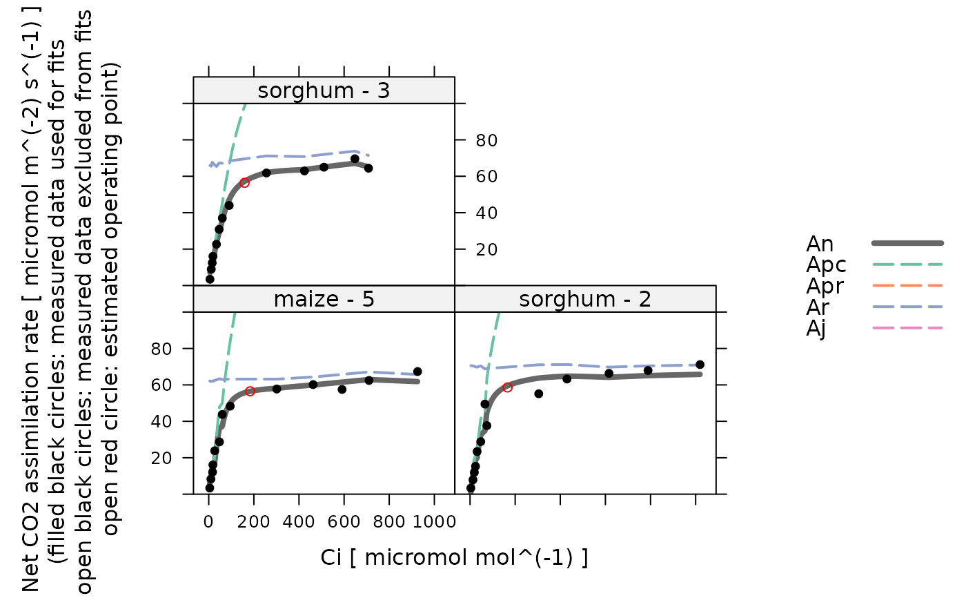
The resulting plot will show curves for the fitted rates An, Apr, Apc, and Ar, along with points for the measured values of A, and (optionally) the estimated operating point. The x-axis can be set to either Ci or PCm.

Internally, this function uses xyplot to perform the plotting. Optionally, additional arguments can be passed to xyplot. These should typically be limited to things like xlim, ylim, main, and grid, since many other xyplot arguments will be set internally (such as xlab, ylab, auto, and others).

See the help file for fit_c4_aci for an example using this function.

Value

A trellis object created by lattice::xyplot.

Examples

# Read an example Licor file included in the PhotoGEA package
licor_file <- read_gasex_file(
  PhotoGEA_example_file_path('c4_aci_1.xlsx')
)

# Define a new column that uniquely identifies each curve
licor_file[, 'species_plot'] <-
  paste(licor_file[, 'species'], '-', licor_file[, 'plot'] )

# Organize the data
licor_file <- organize_response_curve_data(
    licor_file,
    'species_plot',
    c(9, 10, 16),
    'CO2_r_sp'
)

# Calculate temperature-dependent values of C4 photosynthetic parameters
licor_file <- calculate_temperature_response(licor_file, c4_temperature_param_vc)

# Calculate the total pressure in the Licor chamber
licor_file <- calculate_total_pressure(licor_file)

# For these examples, we will use a faster (but sometimes less reliable)
# optimizer so they run faster
optimizer <- optimizer_nmkb(1e-7)

# Fit all curves in the data set
aci_results <- consolidate(by(
  licor_file,
  licor_file[, 'species_plot'],
  fit_c4_aci,
  Ca_atmospheric = 420,
  optim_fun = optimizer
))

# View the fits for each species / plot
plot_c4_aci_fit(aci_results, 'species_plot', 'Ci', ylim = c(0, 100))