Make an initial guess of FvCB model parameter values for one curve
initial_guess_c3_aci.RdCreates a function that makes an initial guess of FvCB model parameter values
for one curve. This function is used internally by fit_c3_aci.
Values estimated by this guessing function should be considered inaccurate, and should always be improved upon by an optimizer.
Usage
initial_guess_c3_aci(
    alpha_g,
    alpha_old,
    alpha_s,
    alpha_t,
    Gamma_star_at_25,
    gmc_at_25,
    Kc_at_25,
    Ko_at_25,
    cc_threshold_rl = 100,
    Wj_coef_C = 4.0,
    Wj_coef_Gamma_star = 8.0,
    a_column_name = 'A',
    ci_column_name = 'Ci',
    gamma_star_norm_column_name = 'Gamma_star_norm',
    gmc_norm_column_name = 'gmc_norm',
    j_norm_column_name = 'J_norm',
    kc_norm_column_name = 'Kc_norm',
    ko_norm_column_name = 'Ko_norm',
    oxygen_column_name = 'Oxygen',
    rl_norm_column_name = 'RL_norm',
    total_pressure_column_name = 'total_pressure',
    tp_norm_column_name = 'Tp_norm',
    vcmax_norm_column_name = 'Vcmax_norm',
    debug_mode = FALSE
  )
Arguments
- alpha_g
A dimensionless parameter where
0 <= alpha_g <= 1, representing the proportion of glycolate carbon taken out of the photorespiratory pathway as glycine.alpha_gis often assumed to be 0. Ifalpha_gis not a number, then there must be a column inrc_exdfcalledalpha_gwith appropriate units. A numeric value supplied here will overwrite the values in thealpha_gcolumn ofrc_exdfif it exists.- alpha_old
A dimensionless parameter where
0 <= alpha_old <= 1, representing the fraction of remaining glycolate carbon not returned to the chloroplast after accounting for carbon released as CO2.alpha_oldis often assumed to be 0. Ifalpha_oldis not a number, then there must be a column inrc_exdfcalledalpha_oldwith appropriate units. A numeric value supplied here will overwrite the values in thealpha_oldcolumn ofrc_exdfif it exists.- alpha_s
A dimensionless parameter where
0 <= alpha_s <= 0.75 * (1 - alpha_g)representing the proportion of glycolate carbon taken out of the photorespiratory pathway as serine.alpha_sis often assumed to be 0. Ifalpha_sis not a number, then there must be a column inrc_exdfcalledalpha_swith appropriate units. A numeric value supplied here will overwrite the values in thealpha_scolumn ofrc_exdfif it exists.- alpha_t
A dimensionless parameter where
0 <= alpha_t <= 1representing the proportion of glycolate carbon taken out of the photorespiratory pathway as CH2-THF.alpha_tis often assumed to be 0. Ifalpha_tis not a number, then there must be a column inrc_exdfcalledalpha_twith appropriate units. A numeric value supplied here will overwrite the values in thealpha_tcolumn ofrc_exdfif it exists.- Gamma_star_at_25
The chloroplastic CO2 concentration at which CO2 gains from Rubisco carboxylation are exactly balanced by CO2 losses from Rubisco oxygenation, at 25 degrees C, expressed in
micromol mol^(-1). IfGamma_star_at_25is not a number, then there must be a column inrc_exdfcalledGamma_star_at_25with appropriate units. A numeric value supplied here will overwrite the values in theGamma_star_at_25column ofrc_exdfif it exists.- gmc_at_25
The mesophyll conductance to CO2 diffusion at 25 degrees C, expressed in
mol m^(-2) s^(-1) bar^(-1). In the absence of other reliable information,gmc_at_25is often assumed to be infinitely large. Ifgmc_at_25is not a number, then there must be a column inrc_exdfcalledgmc_at_25with appropriate units. A numeric value supplied here will overwrite the values in thegmc_at_25column ofrc_exdfif it exists.- Kc_at_25
The Michaelis-Menten constant for Rubisco carboxylation at 25 degrees C, expressed in
micromol mol^(-1). IfKc_at_25is not a number, then there must be a column inrc_exdfcalledKc_at_25with appropriate units. A numeric value supplied here will overwrite the values in theKc_at_25column ofrc_exdfif it exists.- Ko_at_25
The Michaelis-Menten constant for Rubisco oxygenation at 25 degrees C, expressed in
mmol mol^(-1). IfKo_at_25is not a number, then there must be a column inrc_exdfcalledKo_at_25with appropriate units. A numeric value supplied here will overwrite the values in theKo_at_25column ofrc_exdfif it exists.- cc_threshold_rl
An upper cutoff value for the chloroplast CO2 concentration in
micromol mol^(-1)to be used when estimatingRL.- Wj_coef_C
A coefficient in the equation for RuBP-regeneration-limited carboxylation, whose value depends on assumptions about the NADPH and ATP requirements of RuBP regeneration; see
calculate_c3_assimilationfor more information.- Wj_coef_Gamma_star
A coefficient in the equation for RuBP-regeneration-limited carboxylation, whose value depends on assumptions about the NADPH and ATP requirements of RuBP regeneration; see
calculate_c3_assimilationfor more information.- a_column_name
The name of the column in
rc_exdfthat contains the net assimilation inmicromol m^(-2) s^(-1).- ci_column_name
The name of the column in
rc_exdfthat contains the intercellular CO2 concentration inmicromol mol^(-1).- gamma_star_norm_column_name
The name of the column in
rc_exdfthat contains the normalizedGamma_starvalues (with units ofnormalized to Gamma_star at 25 degrees C).- gmc_norm_column_name
The name of the column in
rc_exdfthat contains the normalized mesophyll conductance values (with units ofnormalized to gmc at 25 degrees C).- j_norm_column_name
The name of the column in
rc_exdfthat contains the normalizedJvalues (with units ofnormalized to J at 25 degrees C).- kc_norm_column_name
The name of the column in
rc_exdfthat contains the normalizedKcvalues (with units ofnormalized to Kc at 25 degrees C).- ko_norm_column_name
The name of the column in
rc_exdfthat contains the normalizedKovalues (with units ofnormalized to Ko at 25 degrees C).- oxygen_column_name
The name of the column in
rc_exdfthat contains the concentration of O2 in the ambient air, expressed as a percentage (commonly 21% or 2%); the units must bepercent.- rl_norm_column_name
The name of the column in
rc_exdfthat contains the normalizedRLvalues (with units ofnormalized to RL at 25 degrees C).- total_pressure_column_name
The name of the column in
rc_exdfthat contains the total pressure inbar.- tp_norm_column_name
The name of the column in
rc_exdfthat contains the normalizedTpvalues (with units ofnormalized to Tp at 25 degrees C).- vcmax_norm_column_name
The name of the column in
rc_exdfthat contains the normalizedVcmaxvalues (with units ofnormalized to Vcmax at 25 degrees C).- debug_mode
A logical (
TRUEorFALSE) variable indicating whether to operate in debug mode. In debug mode, information about the linear fit used to estimateRLis printed; this can be helpful when troubleshooting issues with a particular curve.
Details
Here we estimate values of J_at_25, RL_at_25, Tp_at_25,
and Vcmax_at_25 from a measured C3 CO2 response curve. It is difficult
to estimate values of alpha_g, alpha_old, alpha_s,
alpha_t, Gamma_star_at_25, gmc_at_25, Kc_at_25,
Ko_at_25 from a curve, so they must be supplied beforehand. For more
information about these parameters, see the documentation for
calculate_c3_assimilation.
Estimating RL: Regardless of which process is limiting at low
Cc, it is always true thatAn = -RLwhenCc = Gamma_star_agt. Here we make a linear fit of the measuredAnvs.Ccvalues whereCcis belowcc_threshold_rl, and evaluate it at atCc = Gamma_star_agtto estimateRL. If there are fewer than two points withCc <= cc_threshold_rl, the fit cannot be made, and we use a typical value instead (1.0micromol m^(-2) s^(-1)). Likewise, if the linear fit predicts a negative orNAvalue forRL, we use the same typical value instead.Estimating Vc: Once an estimate for
RLhas been found, the RuBP carboxylation rateVccan be estimated usingVc = (An + RL) / (1 - Gamma_star_agt / Cc). This is useful for the remaining parameter estimates.Estimating Vcmax: An estimate for
Vcmaxcan be obtained by solving the equation forWcforVcmax, and evaluating it withWc = Vcas estimated above. In the rubisco-limited part of the curve,Vc = Wcand the estimated values ofVcmaxshould be reasonable. In other parts of the curve,Wcis not the limiting rate, soVc < Wc. Consequently, the estimated values ofVcmaxin these parts of the curve will be smaller. So, to make an overall estimate, we choose the the largest estimatedVcmaxvalue.Estimating J and Tp: Estimates for these parameters can be made using the equations for
WjandWp, similar to the approach followed forVcmax.
For the parameter values estimated above, the values of RL_norm,
Vcmax_norm, and J_norm are used to convert the values at leaf
temperature to the values at 25 degrees C.
Value
A function with one input argument rc_exdf, which should be an
exdf object representing one C3 CO2 response curve. The return value of
this function will be a numeric vector with twelve elements, representing the
values of alpha_g, alpha_old, alpha_s, alpha_t,
Gamma_star_at_25, gmc_at_25, J_at_25, Kc_at_25,
Ko_at_25, RL_at_25, Tp_at_25, and Vcmax_at_25 (in
that order).
Examples
# Read an example Licor file included in the PhotoGEA package
licor_file <- read_gasex_file(
PhotoGEA_example_file_path('c3_aci_1.xlsx')
)
# Define a new column that uniquely identifies each curve
licor_file[, 'species_plot'] <-
paste(licor_file[, 'species'], '-', licor_file[, 'plot'] )
# Organize the data
licor_file <- organize_response_curve_data(
licor_file,
'species_plot',
c(9, 10, 16),
'CO2_r_sp'
)
# Calculate the total pressure in the Licor chamber
licor_file <- calculate_total_pressure(licor_file)
# Calculate temperature-dependent values of C3 photosynthetic parameters
licor_file <- calculate_temperature_response(licor_file, c3_temperature_param_bernacchi)
# Create the guessing function; here we set:
# - All alpha values to 0
# - Gamma_star_at_25 to 40 micromol / mol
# - gmc to infinity
# - Kc_at_25 to 400 micromol / mol
# - Ko_at_25 to 275 mmol / mol
guessing_func <- initial_guess_c3_aci(
alpha_g = 0,
alpha_old = 0,
alpha_s = 0,
alpha_t = 0,
Gamma_star = 40,
gmc_at_25 = Inf,
Kc_at_25 = 400,
Ko_at_25 = 275
)
# Apply it and see the initial guesses for each curve
print(by(licor_file, licor_file[, 'species_plot'], guessing_func))
#> $`soybean - 5a`
#> [1] 0.0000000 0.0000000 0.0000000 0.0000000 40.0000000 Inf
#> [7] 207.7214921 400.0000000 275.0000000 0.8878856 14.9438964 164.3471181
#>
#> $`tobacco - 1`
#> [1] 0.000000 0.000000 0.000000 0.000000 40.000000 Inf
#> [7] 246.842674 400.000000 275.000000 1.325456 18.385860 343.034039
#>
#> $`tobacco - 2`
#> [1] 0.000000 0.000000 0.000000 0.000000 40.000000 Inf
#> [7] 220.413963 400.000000 275.000000 1.197193 17.291378 155.417962
#>
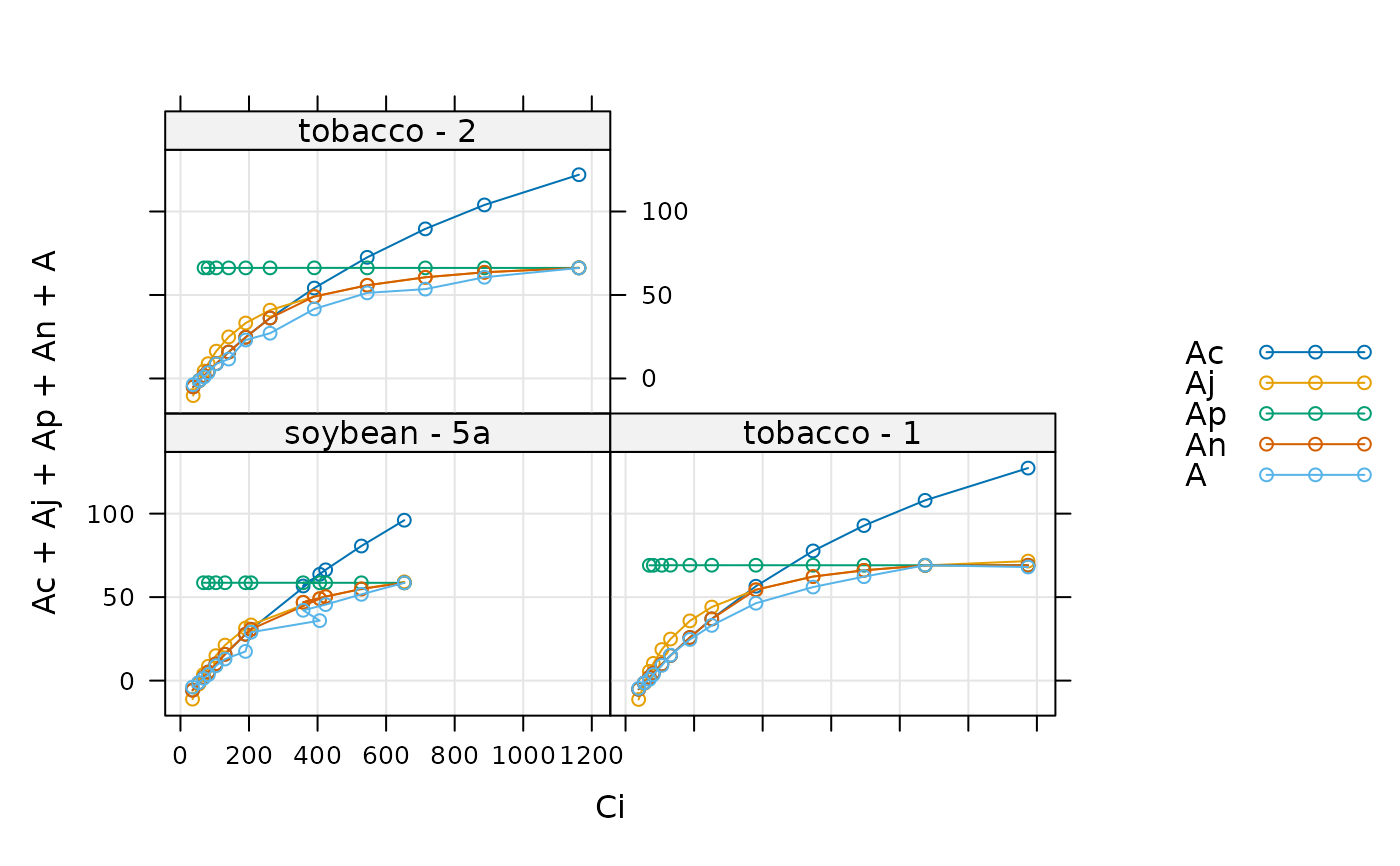
# A simple way to visualize the guesses is to "fit" the curves using the null
# optimizer, which simply returns the initial guess
aci_results <- consolidate(by(
licor_file,
licor_file[, 'species_plot'],
fit_c3_aci,
fit_options = list(alpha_old = 0),
optim_fun = optimizer_null(),
remove_unreliable_param = 0
))
plot_c3_aci_fit(aci_results, 'species_plot', 'Ci')