Fits a C3 assimilation model to an A-Ci + CF curve — fit_c3_variable

Fits the Farquhar-von-Caemmerer-Berry + Variable J model to an experimentally measured C3 A-Ci + CF curve.

It is possible to fit the following parameters: alpha_g, alpha_old, alpha_s, alpha_t, Gamma_star_at_25, J_at_25, Kc_at_25, Ko_at_25 RL_at_25, tau, Tp_at_25, and Vcmax_at_25.

By default, only a subset of these parameters are actually fit: alpha_old, J_at_25, RL_at_25, tau, Tp_at_25, and Vcmax_at_25. This can be altered using the fit_options argument, as described below.

Best-fit parameters are found using maximum likelihood fitting, where the optimizer (optim_fun) is used to minimize the error function (defined by error_function_c3_variable_j).

Once best-fit parameters are found, confidence intervals are calculated using confidence_intervals_c3_variable_j, and unreliable parameter estimates are removed.

For temperature-dependent parameters, best-fit values and confidence intervals are returned at 25 degrees C and at leaf temperature.

See below for more details.

Usage

fit_c3_variable_j(
    replicate_exdf,
    Ca_atmospheric = NA,
    a_column_name = 'A',
    ca_column_name = 'Ca',
    ci_column_name = 'Ci',
    etr_column_name = 'ETR',
    gamma_star_norm_column_name = 'Gamma_star_norm',
    j_norm_column_name = 'J_norm',
    kc_norm_column_name = 'Kc_norm',
    ko_norm_column_name = 'Ko_norm',
    oxygen_column_name = 'Oxygen',
    phips2_column_name = 'PhiPS2',
    qin_column_name = 'Qin',
    rl_norm_column_name = 'RL_norm',
    total_pressure_column_name = 'total_pressure',
    tp_norm_column_name = 'Tp_norm',
    vcmax_norm_column_name = 'Vcmax_norm',
    sd_A = 'RMSE',
    Wj_coef_C = 4.0,
    Wj_coef_Gamma_star = 8.0,
    optim_fun = optimizer_deoptim(400),
    lower = list(),
    upper = list(),
    fit_options = list(),
    cj_crossover_min = NA,
    cj_crossover_max = NA,
    require_positive_gmc = 'positive_a',
    gmc_max = Inf,
    check_j = TRUE,
    relative_likelihood_threshold = 0.147,
    hard_constraints = 0,
    calculate_confidence_intervals = TRUE,
    remove_unreliable_param = 2,
    debug_mode = FALSE,
    ...
  )

Arguments

replicate_exdf: An exdf object representing one CO2 response curve.
Ca_atmospheric: The atmospheric CO2 concentration (with units of micromol mol^(-1)); this will be used by estimate_operating_point to estimate the operating point. A value of NA disables this feature.
a_column_name: The name of the column in replicate_exdf that contains the net assimilation in micromol m^(-2) s^(-1).
ca_column_name: The name of the column in replicate_exdf that contains the ambient CO2 concentration in micromol mol^(-1). If values of Ca are not available, they can be set to NA. In this case, it will not be possible to estimate the operating point, and apply_gm will not be able to calculate the CO2 drawdown across the stomata.
ci_column_name: The name of the column in replicate_exdf that contains the intercellular CO2 concentration in micromol mol^(-1).
etr_column_name: The name of the column in rc_exdf that contains the electron transport rate as estimated by the measurement system in micromol m^(-2) s^(-1).
gamma_star_norm_column_name: The name of the column in replicate_exdf that contains the normalized Gamma_star values (with units of normalized to Gamma_star at 25 degrees C).
j_norm_column_name: The name of the column in replicate_exdf that contains the normalized J values (with units of normalized to J at 25 degrees C).
kc_norm_column_name: The name of the column in replicate_exdf that contains the normalized Kc values (with units of normalized to Kc at 25 degrees C).
ko_norm_column_name: The name of the column in replicate_exdf that contains the normalized Ko values (with units of normalized to Ko at 25 degrees C).
oxygen_column_name: The name of the column in replicate_exdf that contains the concentration of O2 in the ambient air, expressed as a percentage (commonly 21% or 2%); the units must be percent.
phips2_column_name: The name of the column in replicate_exdf that contains values of the operating efficiency of photosystem II (dimensionless).
qin_column_name: The name of the column in replicate_exdf that contains values of the incident photosynthetically active flux density in micromol m^(-2) s^(-1).
rl_norm_column_name: The name of the column in replicate_exdf that contains the normalized RL values (with units of normalized to RL at 25 degrees C).
total_pressure_column_name: The name of the column in replicate_exdf that contains the total pressure in bar.
tp_norm_column_name: The name of the column in replicate_exdf that contains the normalized Tp values (with units of normalized to Tp at 25 degrees C).
vcmax_norm_column_name: The name of the column in replicate_exdf that contains the normalized Vcmax values (with units of normalized to Vcmax at 25 degrees C).
sd_A: A value of the standard deviation of measured A values, or the name of a method for determining the deviation; currently, the only supported option is 'RMSE'.
Wj_coef_C: A coefficient in the equation for RuBP-regeneration-limited carboxylation, whose value depends on assumptions about the NADPH and ATP requirements of RuBP regeneration; see calculate_c3_assimilation for more information.
Wj_coef_Gamma_star: A coefficient in the equation for RuBP-regeneration-limited carboxylation, whose value depends on assumptions about the NADPH and ATP requirements of RuBP regeneration; see calculate_c3_assimilation for more information.
optim_fun: An optimization function that accepts the following input arguments: an initial guess, an error function, lower bounds, and upper bounds. It should return a list with the following elements: par, convergence, feval, and convergence_msg. The default option is an evolutionary optimizer that runs slow but tends to find good fits for most curves. optimizer_nmkb can also be used; it is faster, but doesn't always find a good fit.
lower: A list of named numeric elements representing lower bounds to use when fitting. Values supplied here override the default values (see details below). For example, lower = list(Vcmax_at_25 = 10) sets the lower limit for Vcmax_at_25 to 10 micromol / m^2 / s.
upper: A list of named numeric elements representing upper bounds to use when fitting. Values supplied here override the default values (see details below). For example, upper = list(Vcmax_at_25 = 200) sets the upper limit for Vcmax_at_25 to 200 micromol / m^2 / s.
fit_options: A list of named elements representing fit options to use for each parameter. Values supplied here override the default values (see details below). Each element must be 'fit', 'column', or a numeric value. A value of 'fit' means that the parameter will be fit; a value of 'column' means that the value of the parameter will be taken from a column in replicate_exdf of the same name; and a numeric value means that the parameter will be set to that value. For example, fit_options = list(alpha_g = 0, Vcmax_at_25 = 'fit', Tp_at_25 = 'column') means that alpha_g will be set to 0, Vcmax_at_25 will be fit, and Tp_at_25 will be set to the values in the Tp_at_25 column of replicate_exdf.
cj_crossover_min: To be passed to error_function_c3_variable_j.
cj_crossover_max: To be passed to error_function_c3_variable_j.
require_positive_gmc: To be passed to error_function_c3_variable_j.
gmc_max: To be passed to error_function_c3_variable_j.
check_j: To be passed to error_function_c3_variable_j.
relative_likelihood_threshold: To be passed to confidence_intervals_c3_variable_j when calculate_confidence_intervals is TRUE.
hard_constraints: To be passed to calculate_c3_assimilation and calculate_c3_variable_j; see those functions for more details.
calculate_confidence_intervals: A logical value indicating whether or not to estimate confidence intervals for the fitting parameters using confidence_intervals_c3_variable_j.
remove_unreliable_param: An integer value indicating the rules to use when identifying and removing unreliable parameter estimates. A value of 2 is the most conservative option. A value of 0 disables this feature, which is not typically recommended. It is also possible to directly specify the trust values to remove; for example, 'unreliable (process never limiting)' is equivalent to 1. See below for more details.
debug_mode: A logical (TRUE or FALSE) variable indicating whether to operate in debug mode. In debug mode, information about replicate_exdf, the initial guess, each guess supplied from the optimizer, and the final outcome is printed; this can be helpful when troubleshooting issues with a particular curve.
...: Additional arguments to be passed to calculate_c3_assimilation.

Details

This function calls calculate_c3_variable_j and calculate_c3_assimilation to calculate values of net assimilation. The user-supplied optimization function is used to vary the values of alpha_g, alpha_old, alpha_s, alpha_t, Gamma_star_at_25, J_at_25, Kc_at_25, Ko_at_25, RL_at_25, tau, Tp_at_25, and Vcmax_at_25 to find ones that best reproduce the experimentally measured values of net assimilation. By default, the following options are used for the fits:

alpha_g: lower = 0, upper = 10, fit_option = 0
alpha_old: lower = 0, upper = 10, fit_option = 'fit'
alpha_s: lower = 0, upper = 10, fit_option = 0
alpha_t: lower = 0, upper = 10, fit_option = 0
Gamma_star_at_25: lower = -20, upper = 200, fit_option = 'column'
J_at_25: lower = -50, upper = 1000, fit_option = 'fit'
Kc_at_25: lower = -50, upper = 1000, fit_option = 'column'
Ko_at_25: lower = -50, upper = 1000, fit_option = 'column'
RL_at_25: lower = -10, upper = 100, fit_option = 'fit'
tau: lower = -10, upper = 10, fit_option = 'fit'
Tp_at_25: lower = -10, upper = 100, fit_option = 'fit'
Vcmax_at_25: lower = -50, upper = 1000, fit_option = 'fit'

With these settings, all "new" alpha parameters are set to 0; values of Gamma_star_at_25, Kc_at_25, and Ko_at_25 are taken from the Gamma_star_at_25, Kc_at_25, and Ko_at_25 columns of replicate_exdf; and the other parameters are fit during the process (see fit_options above). The bounds are chosen liberally to avoid any bias.

An initial guess for the parameters is generated by calling initial_guess_c3_variable_j as follows:

cc_threshold_rl is set to 100 micromol / mol.
If alpha_g is being fit, the alpha_g argument of initial_guess_c3_variable_j is set to 0.5; otherwise, the argument is set to the value specified by the fit options.
If alpha_old is being fit, the alpha_old argument of initial_guess_c3_variable_j is set to 0.5; otherwise, the argument is set to the value specified by the fit options.
if alpha_s is being fit, the alpha_s argument of initial_guess_c3_variable_j is set to 0.3 * (1 - alpha_g); otherwise, the argument is set to the value specified by the fit options.
if alpha_t is being fit, the alpha_t argument of initial_guess_c3_variable_j is set to 0; otherwise, the argument is set to the value specified by the fit options.
If Gamma_star_at_25 is being fit, the Gamma_star_at_25 argument of initial_guess_c3_variable_j is set to 40; otherwise, the argument is set to the value specified by the fit options.
If Kc_at_25 is being fit, the Kc_at_25 argument of initial_guess_c3_variable_j is set to 400; otherwise, the argument is set to the value specified by the fit options.
If Ko_at_25 is being fit, the Ko_at_25 argument of initial_guess_c3_variable_j is set to 275; otherwise, the argument is set to the value specified by the fit options.

Note that any fixed values specified in the fit options will override the values returned by the guessing function.

The fit is made by creating an error function using error_function_c3_variable_j and minimizing its value using optim_fun, starting from the initial guess described above. The optimizer_deoptim optimizer is used by default since it has been found to reliably return great fits. However, it is a slow optimizer. If speed is important, consider reducing the number of generations or using optimizer_nmkb, but be aware that this optimizer is more likely to get stuck in a local minimum.

The photosynthesis model used here is not smooth in the sense that small changes in the input parameters do not necessarily cause changes in its outputs. This is related to the final step in the calculations, where the overall assimilation rate is taken to be the minimum of three enzyme-limited rates. For example, if the assimilation rate is never phosphate-limited, modifying Tp_at_25 will not change the model's outputs. For this reason, derivative-based optimizers tend to struggle when fitting C3 A-Ci curves. Best results are obtained using derivative-free methods.

Sometimes the optimizer may choose a set of parameter values where one or more of the potential limiting carboxylation rates (Wc, Wj, or Wp) is never the smallest rate. In this case, the corresponding parameter estimates (Vcmax, J, or alpha_old & Tp) will be severely unreliable. This will be indicated by a value of 'unreliable (process never limiting)' in the corresponding trust column (for example, Vcmax_trust). If remove_unreliable_param is 1 or larger, then such parameter estimates (and the corresponding rates) will be replaced by NA in the fitting results.

It is also possible that the upper limit of the confidence interval for a parameter is infinity; this indicates a potentially unreliable parameter estimate. This will be indicated by a value of 'unreliable (infinite upper limit)' in the corresponding trust column (for example, Vcmax_trust). If remove_unreliable_param is 2 or larger, then such parameter estimates (but not the corresponding rates) will be replaced by NA in the fitting results.

The trust value for fully reliable parameter estimates is set to 'reliable' and they will never be replaced by NA.

Once the best-fit parameters have been determined, this function also estimates the operating value of `Cc from the atmospheric CO2 concentration atmospheric_ca using estimate_operating_point, and then uses that value to estimate the modeled An at the operating point via calculate_c3_assimilation. It also estimates the Akaike information criterion (AIC).

This function assumes that replicate_exdf represents a single C3 A-Ci curve. To fit multiple curves at once, this function is often used along with by.exdf and consolidate.

Value

A list with two elements:

fits: An exdf object including the original contents of replicate_exdf along with several new columns:
- The fitted values of net assimilation will be stored in a column whose name is determined by appending '_fit' to the end of a_column_name; typically, this will be 'A_fit'.
- Residuals (measured - fitted) will be stored in a column whose name is determined by appending '_residuals' to the end of a_column_name; typically, this will be 'A_residuals'.
- Values of fitting parameters at 25 degrees C will be stored in the Gamma_star_at_25, J_at_25, Kc_at_25, Ko_at_25, RL_at_25, Tp_at_25, and Vcmax_at_25 columns.
- The other outputs from calculate_c3_variable_j and calculate_c3_assimilation will be stored in columns with the usual names: alpha_g, alpha_old, alpha_s, alpha_t, Gamma_star_tl, J_tl, Kc_tl, Ko_tl, RL_tl, tau, Tp_tl, Vcmax_tl, Ac, Aj, Ap, gmc, J_F, and Cc.
fits_interpolated: An exdf object including the calculated assimilation rates at a fine spacing of Ci values (step size of 1 micromol mol^(-1)).
parameters: An exdf object including the identifiers, fitting parameters, and convergence information for the A-Ci curve:
- The number of points where An = Ac, An = Aj, and An = Ap are stored in the n_Ac_limiting, n_Aj_limiting, and n_Ap_limiting columns.
- The best-fit values are stored in the alpha_g, alpha_old, alpha_s, alpha_t, Gamma_star_at_25, J_at_25, Kc_at_25, Ko_at_25, RL_at_25, tau, Tp_at_25, and Vcmax_at_25 columns. If calculate_confidence_intervals is TRUE, upper and lower limits for each of these parameters will also be included.
- For parameters that depend on leaf temperature, the average leaf-temperature-dependent values are stored in Gamma_star_tl_avg, J_tl_avg, Kc_tl_avg, Ko_tl_avg, RL_tl_avg, Tp_tl_avg, and Vcmax_tl_avg.
- Information about the operating point is stored in operating_Cc, operating_Ci, operating_An, and operating_An_model.
- The convergence column indicates whether the fit was successful (==0) or if the optimizer encountered a problem (!=0).
- The feval column indicates how many cost function evaluations were required while finding the optimal parameter values.
- The residual stats as returned by residual_stats are included as columns with the default names: dof, RSS, RMSE, etc.
- The Akaike information criterion is included in the AIC column.

Examples

# Read an example Licor file included in the PhotoGEA package
licor_file <- read_gasex_file(
  PhotoGEA_example_file_path('c3_aci_1.xlsx')
)

# Define a new column that uniquely identifies each curve
licor_file[, 'species_plot'] <-
  paste(licor_file[, 'species'], '-', licor_file[, 'plot'] )

# Organize the data
licor_file <- organize_response_curve_data(
    licor_file,
    'species_plot',
    c(9, 10, 16),
    'CO2_r_sp'
)

# Calculate the total pressure in the Licor chamber
licor_file <- calculate_total_pressure(licor_file)

# Calculate temperature-dependent values of C3 photosynthetic parameters
licor_file <- calculate_temperature_response(licor_file, c3_temperature_param_bernacchi)

# For these examples, we will use a faster (but sometimes less reliable)
# optimizer so they run faster
optimizer <- optimizer_nmkb(1e-7)

# Fit just one curve from the data set (it is rare to do this).
one_result <- fit_c3_variable_j(
  licor_file[licor_file[, 'species_plot'] == 'tobacco - 1', , TRUE],
  Ca_atmospheric = 420,
  optim_fun = optimizer
)

# Fit all curves in the data set (it is more common to do this).
aci_results <- consolidate(by(
  licor_file,
  licor_file[, 'species_plot'],
  fit_c3_variable_j,
  Ca_atmospheric = 420,
  optim_fun = optimizer
))

# View the fitting parameters for each species / plot
col_to_keep <- c(
  'species', 'plot',                                       # identifiers
  'n_Ac_limiting', 'n_Aj_limiting', 'n_Ap_limiting',       # number of points where
                                                           #   each process is limiting
  'tau', 'Tp_at_25',                                       # parameters with temperature response
  'J_at_25', 'RL_at_25', 'Vcmax_at_25',                    # parameters scaled to 25 degrees C
  'J_tl_avg', 'RL_tl_avg', 'Vcmax_tl_avg',                 # average temperature-dependent values
  'operating_Ci', 'operating_An', 'operating_An_model',    # operating point info
  'dof', 'RSS', 'MSE', 'RMSE', 'RSE',                      # residual stats
  'convergence', 'convergence_msg', 'feval', 'optimum_val' # convergence info
)

aci_results$parameters[ , col_to_keep, TRUE]
#> 
#> Converting an `exdf` object to a `data.frame` before printing
#> 
#>   species [UserDefCon] (NA) plot [UserDefCon] (NA)
#> 1                   soybean                     5a
#> 2                   tobacco                      1
#> 3                   tobacco                      2
#>   n_Ac_limiting [identify_c3_unreliable_points] ()
#> 1                                                9
#> 2                                               10
#> 3                                                9
#>   n_Aj_limiting [identify_c3_unreliable_points] ()
#> 1                                                3
#> 2                                                3
#> 3                                                4
#>   n_Ap_limiting [identify_c3_unreliable_points] ()
#> 1                                                1
#> 2                                                0
#> 3                                                0
#>   tau [fit_c3_variable_j] (micromol m^(-2) s^(-1))
#> 1                                        0.4202992
#> 2                                        0.4202993
#> 3                                        0.4202992
#>   Tp_at_25 [fit_c3_variable_j] (micromol m^(-2) s^(-1))
#> 1                                                    NA
#> 2                                                    NA
#> 3                                                    NA
#>   J_at_25 [fit_c3_variable_j] (micromol m^(-2) s^(-1))
#> 1                                                   NA
#> 2                                                   NA
#> 3                                                   NA
#>   RL_at_25 [fit_c3_variable_j] (micromol m^(-2) s^(-1))
#> 1                                             0.4385477
#> 2                                             0.8163209
#> 3                                             0.7508444
#>   Vcmax_at_25 [fit_c3_variable_j] (micromol m^(-2) s^(-1))
#> 1                                                       NA
#> 2                                                       NA
#> 3                                                       NA
#>   J_tl_avg [fit_c3_variable_j] (micromol m^(-2) s^(-1))
#> 1                                                    NA
#> 2                                                    NA
#> 3                                                    NA
#>   RL_tl_avg [fit_c3_variable_j] (micromol m^(-2) s^(-1))
#> 1                                              0.6193295
#> 2                                              1.1289194
#> 3                                              1.0442328
#>   Vcmax_tl_avg [fit_c3_variable_j] (micromol m^(-2) s^(-1))
#> 1                                                        NA
#> 2                                                        NA
#> 3                                                        NA
#>   operating_Ci [estimate_operating_point] (micromol mol^(-1))
#> 1                                                    264.3297
#> 2                                                    294.7032
#> 3                                                    301.2673
#>   operating_An [estimate_operating_point] (micromol m^(-2) s^(-1))
#> 1                                                         31.00316
#> 2                                                         37.51608
#> 3                                                         31.57904
#>   operating_An_model [fit_c3_variable_j] (micromol m^(-2) s^(-1))
#> 1                                                        30.36569
#> 2                                                        27.28351
#> 3                                                        22.67259
#>   dof [residual_stats] (NA) RSS [residual_stats] ((micromol m^(-2) s^(-1))^2)
#> 1                         7                                          26.70037
#> 2                         7                                         418.25473
#> 3                         7                                         332.87510
#>   MSE [residual_stats] ((micromol m^(-2) s^(-1))^2)
#> 1                                          2.053875
#> 2                                         32.173440
#> 3                                         25.605777
#>   RMSE [residual_stats] (micromol m^(-2) s^(-1))
#> 1                                       1.433135
#> 2                                       5.672164
#> 3                                       5.060215
#>   RSE [residual_stats] (micromol m^(-2) s^(-1))
#> 1                                      1.953033
#> 2                                      7.729856
#> 3                                      6.895911
#>   convergence [fit_c3_variable_j] () convergence_msg [fit_c3_variable_j] ()
#> 1                                  0                 Successful convergence
#> 2                                  0                 Successful convergence
#> 3                                  0                 Successful convergence
#>   feval [fit_c3_variable_j] () optimum_val [fit_c3_variable_j] ()
#> 1                            7                              1e+10
#> 2                            7                              1e+10
#> 3                            7                              1e+10

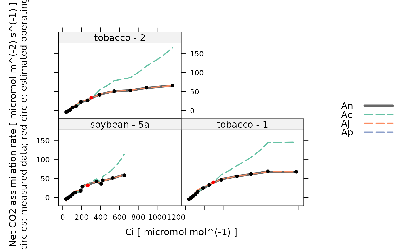
# View the fits for each species / plot
plot_c3_aci_fit(aci_results, 'species_plot', 'Ci')


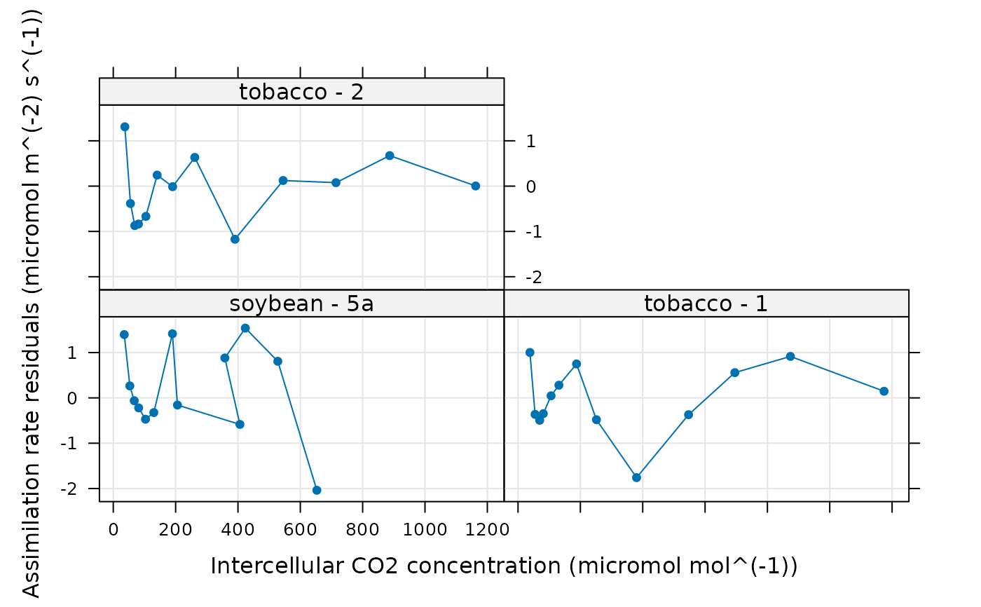
# View the residuals for each species / plot
lattice::xyplot(
  A_residuals ~ Ci | species_plot,
  data = aci_results$fits$main_data,
  type = 'b',
  pch = 16,
  auto = TRUE,
  grid = TRUE,
  xlab = paste0('Intercellular CO2 concentration (', aci_results$fits$units$Ci, ')'),
  ylab = paste0('Assimilation rate residuals (', aci_results$fits$units$A_residuals, ')')
)


# View the estimated mesophyll conductance values for each species / plot
lattice::xyplot(
  gmc ~ Ci | species_plot,
  data = aci_results$fits$main_data,
  type = 'b',
  pch = 16,
  auto = TRUE,
  grid = TRUE,
  xlab = paste0('Intercellular CO2 concentration (', aci_results$fits$units$Ci, ')'),
  ylab = paste0('Mesophyll conductance to CO2 (', aci_results$fits$units$gmc, ')'),
  ylim = c(0, 2)
)


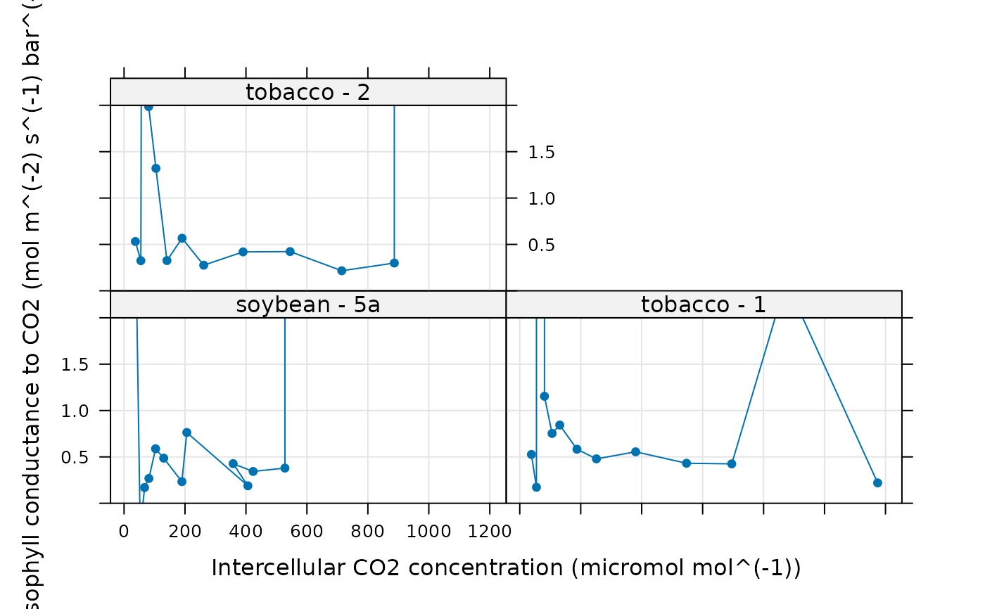# In some of the curves above, there are no points where carboxylation is TPU
# limited. Estimates of Tp are therefore unreliable and are removed.