Plot the results of a C3 CO2 response curve fit — plot_ball_berry

Plots the output from fit_c3_aci or fit_c3_variable_j.

Usage

plot_ball_berry_fit(
    fit_results,
    identifier_column_name,
    bb_index_column_name = 'bb_index',
    gsw_column_name = 'gsw',
    ...
  )

Arguments

fit_results: A list of three exdf objects names fits, parameters, and fits_interpolated, as calculated by fit_c3_aci.
identifier_column_name: The name of a column in each element of fit_results whose value can be used to identify each response curve within the data set; often, this is 'curve_identifier'.
bb_index_column_name: The name of the column in fit_results$fits that contains the Ball-Berry index in mol m^(-2) s^(-1); should be the same value that was passed to fit_ball_berry.
gsw_column_name: The name of the column in fit_results$fits that contains the stomatal conductance to water vapor in mol m^(-2) s^(-1); should be the same value that was passed to fit_ball_berry.
...: Additional arguments to be passed to xyplot.

Details

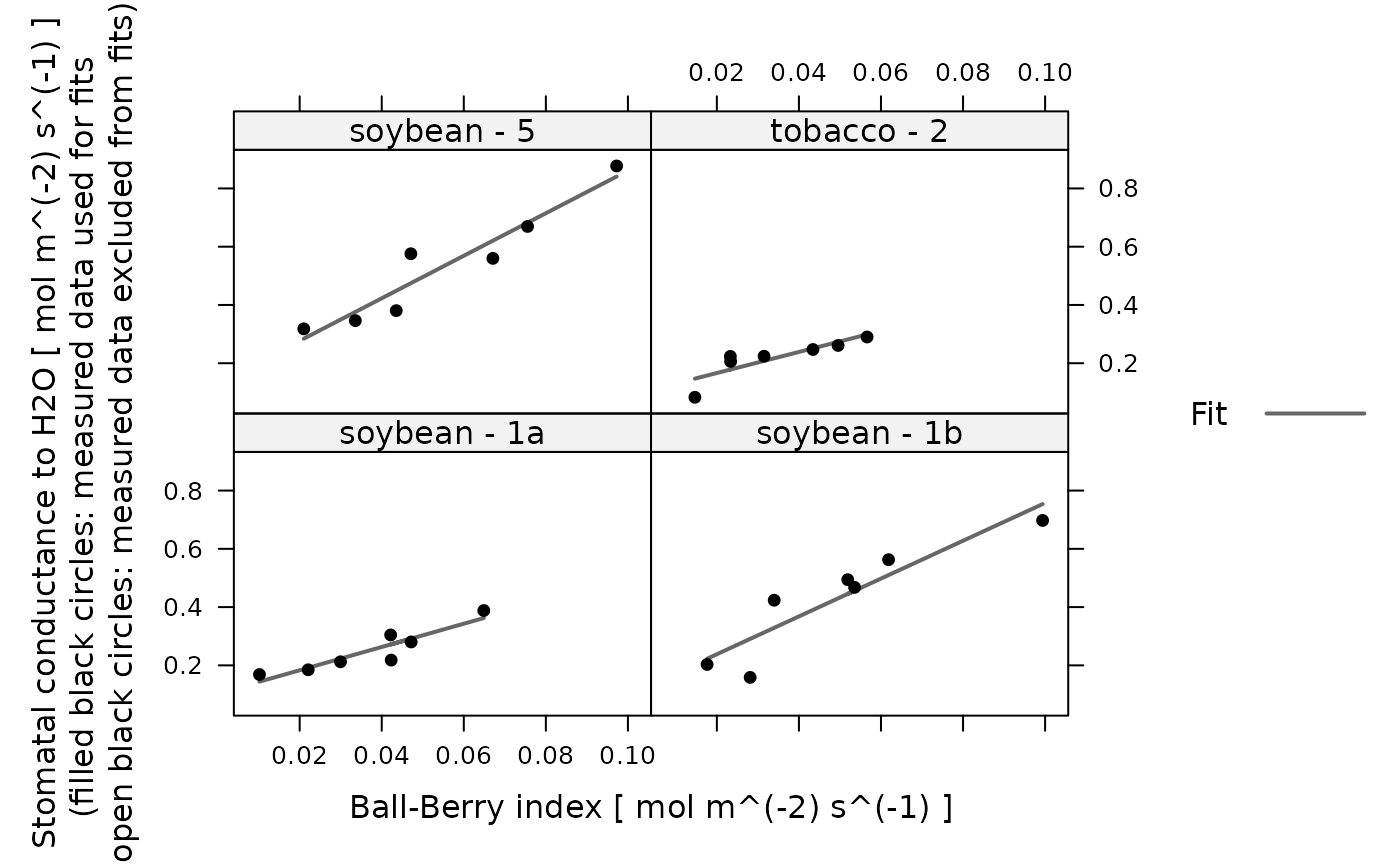
This is a convenience function for plotting the results of a Ball-Berry curve fit. It is typically used for displaying several fits at once, in which case fit_results is actually the output from calling consolidate on a list created by calling by.exdf with FUN = fit_ball_berry.

The resulting plot will show curves for the fitted gsw, along with points for the measured values of gsw.

Internally, this function uses xyplot to perform the plotting. Optionally, additional arguments can be passed to xyplot. These should typically be limited to things like xlim, ylim, main, and grid, since many other xyplot arguments will be set internally (such as xlab, ylab, auto, and others).

See the help file for fit_ball_berry for an example using this function.

Value

A trellis object created by lattice::xyplot.

Examples

# Read an example Licor file included in the PhotoGEA package, calculate
# additional gas properties, calculate the Ball-Berry index, define a new column
# that uniquely identifies each curve, and then perform a fit to extract the
# Ball-Berry parameters from each curve.
licor_file <- read_gasex_file(
  PhotoGEA_example_file_path('ball_berry_1.xlsx')
)

licor_file <- calculate_total_pressure(licor_file)

licor_file <- calculate_gas_properties(licor_file)

licor_file[,'species_plot'] <-
  paste(licor_file[,'species'], '-', licor_file[,'plot'])

licor_file <- calculate_ball_berry_index(licor_file)

# Fit all curves in the data set
bb_results <- consolidate(by(
  licor_file,
  licor_file[, 'species_plot'],
  fit_ball_berry
))

# View the fits for each species / plot
plot_ball_berry_fit(bb_results, 'species_plot')