Generate an error function for C4 A-Ci curve fitting with a hyperbola

Creates a function that returns an error value (the negative of the natural logarithm of the likelihood) representing the amount of agreement between modeled and measured An values. When this function is minimized, the likelihood is maximized.

Internally, this function uses link{calculate_c4_assimilation_hyperbola} to calculate assimilation rate values that are compared to the measured ones.

Usage

error_function_c4_aci_hyperbola(
    replicate_exdf,
    fit_options = list(),
    sd_A = 1,
    a_column_name = 'A',
    ci_column_name = 'Ci',
    hard_constraints = 0
  )

Arguments

replicate_exdf

An exdf object representing one CO2 response curve.

fit_options

A list of named elements representing fit options to use for each parameter. Values supplied here override the default values (see details below). Each element must be 'fit', 'column', or a numeric value. A value of 'fit' means that the parameter will be fit; a value of 'column' means that the value of the parameter will be taken from a column in replicate_exdf of the same name; and a numeric value means that the parameter will be set to that value. For example, fit_options = list(rL = 0, Vmax = 'fit', c4_curvature = 'column') means that rL will be set to 0, Vmax will be fit, and c4_curvature will be set to the values in the c4_curvature column of replicate_exdf.

sd_A

The standard deviation of the measured values of the net CO2 assimilation rate, expressed in units of micromol m^(-2) s^(-1). If sd_A is not a number, then there must be a column in exdf_obj called sd_A with appropriate units. A numeric value supplied here will overwrite the values in the sd_A column of exdf_obj if it exists.

a_column_name

The name of the column in replicate_exdf that contains the net assimilation in micromol m^(-2) s^(-1).

ci_column_name

The name of the column in exdf_obj that contains the intercellular CO2 concentration, expressed in micromol mol^(-1).

hard_constraints

To be passed to calculate_c4_assimilation_hyperbola; see that function for more details.

Details

When fitting A-Ci curves, it is necessary to define a function that calculates the likelihood of a given set of c4_curvature, c4_slope, rL, and Vmax values by comparing a model prediction to a measured curve. This function will be passed to an optimization algorithm which will determine the values that produce the smallest error.

The error_function_c4_aci_hyperbola returns such a function, which is based on a particular A-Ci curve and a set of fitting options. It is possible to just fit a subset of the available fitting parameters; by default, all are fit. This behavior can be changed via the fit_options argument.

For practical reasons, the function actually returns values of -ln(L), where L is the likelihood. The logarithm of L is simpler to calculate than L itself, and the minus sign converts the problem from a maximization to a minimization, which is important because most optimizers are designed to minimize a value.

A penalty is added to the error value for any parameter combination where An is not a number, or where calculate_c4_assimilation_hyperbola produces an error.

Value

A function with one input argument guess, which should be a numeric vector representing values of the parameters to be fitted (which are specified by the fit_options input argument.) Each element of guess is the value of one parameter (arranged in alphabetical order.) For example, with the default settings, guess should contain values of c4_curvature, c4_slope, rL, and Vmax (in that order).

Examples

# Read an example Licor file included in the PhotoGEA package
licor_file <- read_gasex_file(
  PhotoGEA_example_file_path('c4_aci_1.xlsx')
)

# Define a new column that uniquely identifies each curve
licor_file[, 'species_plot'] <-
  paste(licor_file[, 'species'], '-', licor_file[, 'plot'] )

# Organize the data
licor_file <- organize_response_curve_data(
    licor_file,
    'species_plot',
    c(9, 10, 16),
    'CO2_r_sp'
)

# Define an error function for one curve from the set
error_fcn <- error_function_c4_aci_hyperbola(
  licor_file[licor_file[, 'species_plot'] == 'maize - 5', , TRUE]
)

# Evaluate the error for c4_curvature = 0.8, c4_slope = 0.5, rL = 1.0, Vmax = 65
error_fcn(c(0.8, 0.5, 1.0, 65))
#> [1] 439.4015

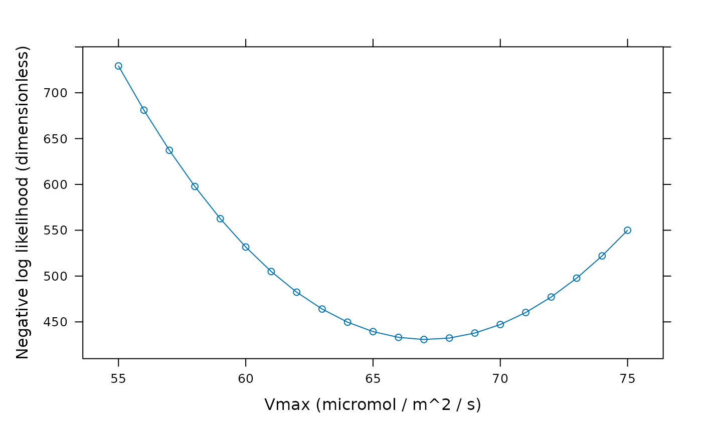
# Make a plot of error vs. Vmax when the other parameters are fixed to
# the values above.
vmax_error_fcn <- function(Vmax) {error_fcn(c(0.8, 0.5, 1.0, Vmax))}
vmax_seq <- seq(55, 75)

lattice::xyplot(
  sapply(vmax_seq, vmax_error_fcn) ~ vmax_seq,
  type = 'b',
  xlab = 'Vmax (micromol / m^2 / s)',
  ylab = 'Negative log likelihood (dimensionless)'
)