Barcharts with error bars

barchart_with_errorbars is a wrapper for lattice::barchart that includes error bars on the chart, while bwplot_wrapper is a simple wrapper for lattice::bwplot that gives it the same function signature as barchart_with_errorbars.

Usage

barchart_with_errorbars(
    Y,
    X,
    eb_width = 0.2,
    eb_lwd = 1,
    eb_col = 'black',
    na.rm = TRUE,
    ...
  )

  bwplot_wrapper(Y, X, ...)

Arguments

Y

A numeric vector.

X

A vector with the same length as Y that can be used as a factor to split Y into one or more distinct subsets.

eb_width

The width of the error bars.

eb_lwd

The line width (thickness) of the error bars.

eb_col

The color of the error bars.

na.rm

A logical value indicating whether or not to remove NA values before calculating means and standard errors.

...

Additional arguments to be passed to lattice::barchart or lattice::bwplot.

Details

The barchart_with_errorbars function uses tapply to calculate the mean and standard error for each subset of Y as determined by the values of X. In other words, means <- tapply(Y, X, mean), and similar for the standard errors. The mean values are represented as bars in the final plot, while the standard error is used to create error bars located at mean +/- standard_error.

The bwplot_wrapper function is a simple wrapper for lattice::bwplot that gives it the same input arguments as barchart_with_errorbars. In other words, the same X and Y vectors can be used to create a barchart using barchart_with_errorbars or a box-whisker plot with bwplot_wrapper.

Value

A trellis object created by lattice::barchart or

lattice::bwplot.

Examples

# Read an example Licor file included in the PhotoGEA package
licor_file <- read_gasex_file(
  PhotoGEA_example_file_path('ball_berry_1.xlsx')
)

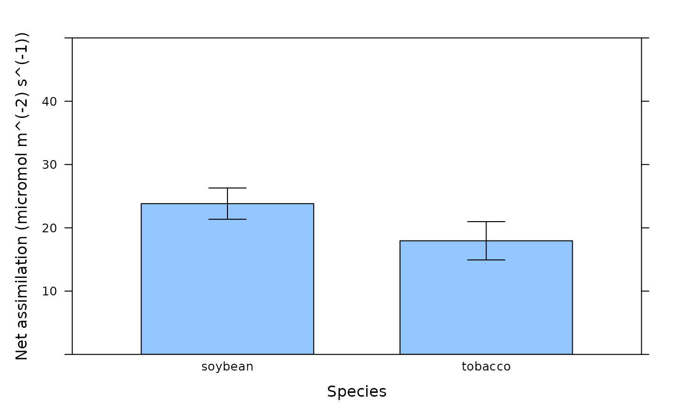
# Plot the average assimilation value for each species. (Note: this is not a
# meaningful calculation since we are combining assimilation values measured
# at different PPFD.)
barchart_with_errorbars(
  licor_file[, 'A'],
  licor_file[, 'species'],
  ylim = c(0, 50),
  xlab = 'Species',
  ylab = paste0('Net assimilation (', licor_file$units$A, ')')
)


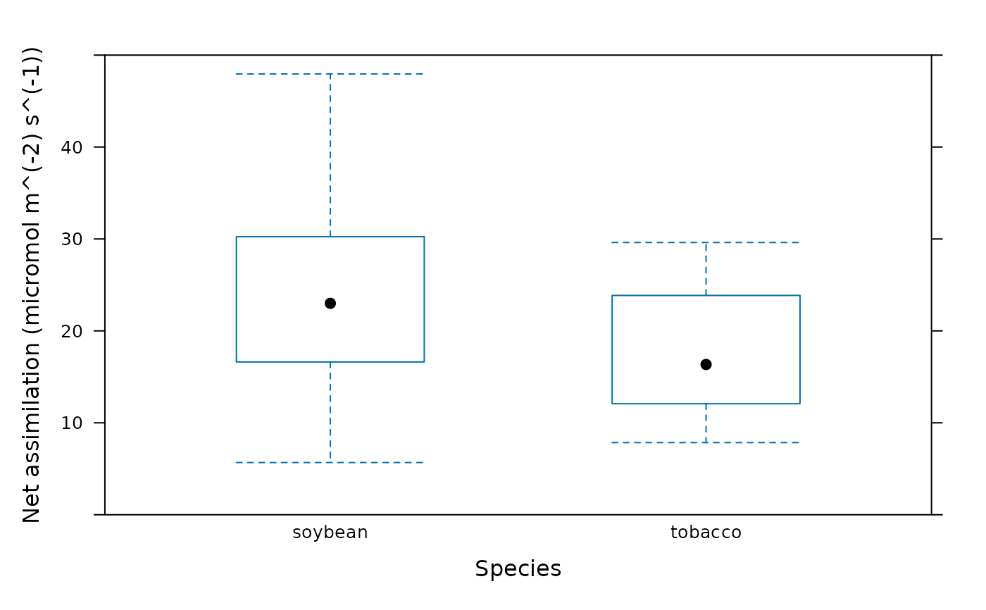
# Make a box-whisker plot using the same data. (Note: this is not a meaningful
# plot since we are combining assimilation values measured at different PPFD.)
bwplot_wrapper(
  licor_file[, 'A'],
  licor_file[, 'species'],
  ylim = c(0, 50),
  xlab = 'Species',
  ylab = paste0('Net assimilation (', licor_file$units$A, ')')
)


# Another way to create the plots. This method illustrates the utility of the
# bwplot_wrapper function.
plot_parameters <- list(
  Y = licor_file[, 'A'],
  X = licor_file[, 'species'],
  ylim = c(0, 50),
  xlab = 'Species',
  ylab = paste0('Net assimilation (', licor_file$units$A, ')')
)
do.call(barchart_with_errorbars, plot_parameters)

do.call(bwplot_wrapper, plot_parameters)